
Overview
Astrometry is the process of determining positions of objects in your field. Modern CCD images and analysis software are able to produce positions accurate to better than one arcsecond when suitable catalogs of comparison objects are used. Here we outline the basic steps you will have to go through in order to obtain accurate positions for objects in your fields. For a more substantial treatment of the background of some of the methods described, see The Handbook of Astronomical Image Processing (HAIP).
The basic idea behind astrometry is to determine the unknown coordinates of objects by comparing their location on an image to the location of a set of objects on the same image whose coordinates are already determined . Assuming such a set of objects with known coordinates exists, you can in principle put any unknown objects on the same coordinate system as the know objects. Fortunately, several star catalogs exist that are suitable for astrometric use. In fact, these catalogs have been compiled just for this purpose. They are listed at the bottom of this page. In addition, most software packages can interact with these catalogs to determine positions of objects in CCD images.
Image Coordinates
There are several different coordinate systems we will use in determining our object coordinates. Some will be familiar, some will likely be new. Each is described in turn. Our treatment follows that found in HAIP, though leaving out much detail.
- Celestial Coordinates (RA,DEC) These are the normal RA and DEC of the Celestial Coordinate system. These are probably what you would like to determine for the objects you are observing.
- Standard Coordinates (X,Y) These are the projection of the RA and DEC of an object onto the tangent plane of the sky, i.e., the plane tangent to the sphere of the sky that intersects the sky at the tangent point (which is usually somewhat offset from the image center). The X coordinate is aligned with RA and the Y coordinate is aligned with DEC. The origin of the standard system is at the tangent point in the image.
- Image Coordinates (x,y) These are the x-y coordinates of an object in your image measured in pixels from the image center (could be in mm if you are using a photograph rather than a CCD image). These differ from standard coordinates because of things like tilt or rotation of the CCD, and also because of possible optical distortions. Ideally the (x,y) and (X,Y) coordinates would be the same.
The trick of astrometry is to turn your image coordinates into celestial coordinates. The usual way this is done is to assume a simple linear transformation between the standard coordinates and the image coordinates, and to determine the coefficients for that transformation. Once that has been done, the standard coordinates for any object can be converted to RA and DEC using straightforward spherical trigonometry. The transformation equations are given below.
Transformation From Image to Celestial Coordinates
The first step is to determine the transformation between image and standard coordinates. The transformation equations are as follows:
X = ax + by + c
Y = dx + ey + f
The symbols (X,Y) and (x,y) have the meanings given above. The constant coefficients a, b, c, d, e and f are to be determined for each image. In principle this can be done using three reference stars of known position to determine the six unknown quantities. Recall that for each star we have two constraints, (X,Y), so three reference stars gives us six constraints on our six unknowns. In practice we typically use more than the minimum three reference stars. In fact, we may use many dozens of reference stars spread across our image, and then determine the “best fit” set of coefficients via a least squares fitting method. See the HAIP or a reference on linear least squares fitting methods to learn how this is done.
Of course, we have not said how to get the (X,Y) coordinates of our reference stars in the first place. This is not difficult. The transformation is derived from spherical trigonometry.

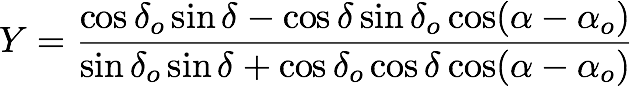
Here the Greek alpha (![]() ) and delta (
) and delta (![]() ) denote RA and DEC, respectively, with the subscript zero (
) denote RA and DEC, respectively, with the subscript zero (![]() ) meaning it is the RA and DEC of the tangent point of our image. With these relations we can compute the (X,Y) position for each of our reference stars, and then use those in our least squares routine.
) meaning it is the RA and DEC of the tangent point of our image. With these relations we can compute the (X,Y) position for each of our reference stars, and then use those in our least squares routine.
The inverse transformation, to take our derived (X,Y) for each object to RA and DEC, is (Note that the HAIP has a sign error in the second equation above, and an incorrect expression for the declination equation below)

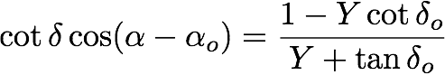
As we mentioned earlier, commonly available astronomical software packages include routines to perform all these transformations for you and to do all the least-squared fitting. However, for those of you who like to write your own code, the relations above will be useful. In any case, computers make pretty straightforward work of these otherwise extremely tedious calculations.
Star Catalogs for Astrometry
The key to performing any of these transformations is having a set of reference objects in each image for which the RA and DEC are already known. There are two star catalogs that are typically used for this purpose, in fact, one of them was created expressly to be reference for accurate astrometry determinations. Both of these catalogs are tied to the Hipparchos satellite astrometric measurements, which are in turn tied to Very Long Baseline Interferometric measurements of the positions of extragalactic radio sources. As such, their positions are extremely well fixed to the sky. The primary difference between them is the number of objects they contain.
The first catalog suitable for fairly accurate astrometry was the HST Guide Star Catalog (GSC). The GSC was compiled to provide a group of stars that could be used to point the Hubble Space Telescope. As such, it was not really intended as an astrometry reference, but because the catalog members have good positions, and especially because there are so many of them, around 15 million, it was taken up as a default astrometric reference. Using the GSC provides position accurate to about one arcsecond, which is good enough for many astrometry applications. The GSC is available online and as a set of CDs.
To do very accurate astrometry you must use the US Naval Observatory astrometric catalogs. These catalogs contain over 500 million stars, which works out to over 12,000 stars per square degree down to R=16. The USNO catalogs have been compiled specifically as a reference for astrometry; the goal was to get adequate coverage around the sky, not to get all the stars to some particular magnitude. The USNO catalogs are available on the web, and subsets of the catalog can be downloaded for any particular region of interest. Generally the USNO catalogs are the best ones to use for your astrometric references, giving positions accurate to around 0.1 arcsecond.
To learn how to use either of these star catalogs with your particular astronomical software package, see the documentation for the package.