
Introduction
|
“The cosmos is all that is, or ever was, or ever will be.”
–Carl Sagan |
With these words, Carl Sagan launched his groundbreaking and historic television series Cosmos in 1979. Since Cosmos first aired on PBS, our understanding of the universe has undergone a revolution, maybe two. In fact, we have gained deeper insights into the nature of the universe over the subsequent four decades than were gleaned in the four millennia prior to that.
Sagan’s TV series was first broadcast at a time when astronomers were on the brink of having
the tools they needed to answer long-standing questions into the nature of the universe, including, How old is the universe? How big is it? What is it made of and how did it come into being? Substantial progress was made answering these questions the years between 1980 and 2020. Here we provide an overview of this progress and discuss some of the basic ideas underlying our current conception of the cosmos.
In The Beginning
Our modern view of the cosmos is usually considered to have begun in the first two or three decades of the 20th century. That is when Albert Einstein developed the General Theory of Relativity and Edwin Hubble made the astounding discovery that the universe is both immense and getting bigger. These two advancements are the foundation upon which current cosmological ideas rest. They are in turn underlain by the work of earlier scientists.
Before any knowledge of the extent and age of the universe could be gained, painstaking work was done to create a basic understanding of stars. This work allowed researchers who came later to make progress learning the scale and history of the universe. Foremost among the early researchers were astronomers at the Harvard College Observatory. They made careful examination of stars and their spectra, and they developed the first large-scale catalogue of stars and stellar properties. While their work had antecedents elsewhere, it was contributions by Williamina Fleming, Antonia Maury and especially Annie J. Cannon, mostly in the last decade of the 19th century, that allowed astronomers to begin to understand the nature of stars.
Skipping ahead two decades, another Harvard astronomer, Cecelia Payne, showed that the composition of the stars is dominated almost entirely – 90% – by hydrogen. Only about a part in ten is helium. Even more astounding, she learned that the remainder, all the other ninety kinds of atoms in the periodic table, comprise only a tiny fraction, far less than a percent in terms of number of atoms. This basic fact is vital for understanding both the workings of the stars and the origin of the universe, and it was completely unknown until the work of Cecelia Payne. We discuss her story and its implications in the pages on The Lives of the Stars.
More pertinent to our current topic is a discovery made by Henrietta Leavitt, also of the Harvard College Observatory. While studying a particular type of variable star (there are many) Leavitt noticed that their period of pulsation is proportional to their absolute brightness. It was one of the most momentous discoveries in the entire history of astronomy, for it allows us to measure the vast distances across the cosmos. Without this knowledge, no understanding of cosmology is possible.
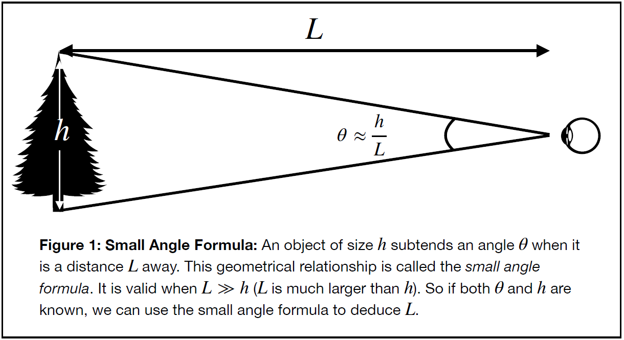
This is because, in general, it is not possible to know the distance to an object by simply looking at it. To infer distance we must know something about it, like it’s size, for instance. Then, by measuring its apparent size (its angular size) and knowing its true size, we can deduce how far away it is using geometry. The method is illustrated in Figure 1, below.
Unfortunately, we cannot use the size of stars to deduce how far away they are. The stars lie at such extreme distances that, with the exception of one or two, they do not have an apparent size. They all appear to be mere points.
However, we do know how bright stars appear to us. In principle, we can use a star’s brightness (its measured intensity, ), along with another geometrical method called the inverse square law, to measure its distance. Figure 2 illustrates how.
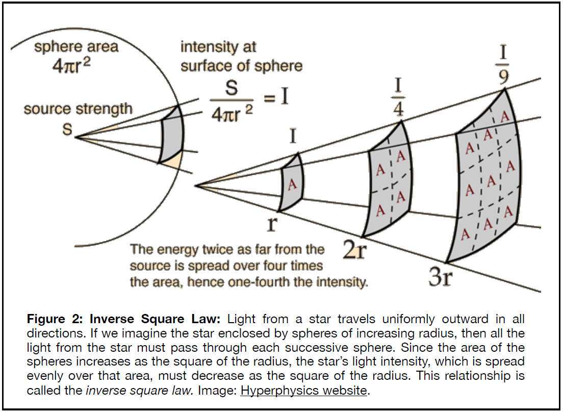
The trouble is, a star’s apparent brightness is affected by two separate things. It could be intrinsically bright, with a large value for S in the diagram above, or it could be nearby, with a small value of r. Either of these will create a large value for the measured brightness, . We cannot usually unravel these two effects from each other.
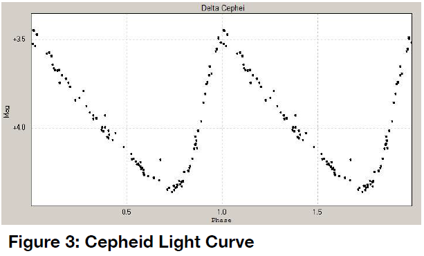
Fortunately, Henrietta Leavitt made a discovery that allows us to overcome the ambiguity. She discovered a particular type of pulsating variable star called a Cepheid variable. These stars get brighter and dimmer in a peculiar manner that makes them easy to distinguish from other kinds of variable stars. A plot of brightness vs. time of the namesake for these stars, Delta Cephei, is shown in Figure 3. Time (in terms of phase) is plotted on the horizontal axis. Brightness (in magnitudes) is plotted vertically.The period of this star is just over five days, but some Cepheid variables have longer periods, and some have shorter periods.
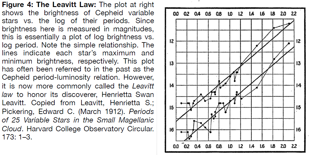
Leavitt was able to study a group of Cepheids in a galaxy called the Small Magellanic Cloud, a dwarf companion of the Milky Way. Since these stars were all in the same tiny galaxy, they were essentially all at the same distance. When she plotted their periods she found an unexpected relationship: the average brightness of a star was proportional to the period of its brightness variations. Leavitt’s relation is shown in Figure 4, a plot of magnitude vs log P, with P the period of variation in days.
If we measure the period of a Cepheid, which is easy to do, we can use the Leavitt law to infer its intrinsic brightness. Once we know the star’s brightness we can combine that measurement with the apparent brightness, and then use the inverse square law to compute its distance.
The Leavitt law is only valid for Cepheid variable stars. Fortunately, Cepheids are fairly common. Some of them are also very, very bright, so it is usually not difficult to find Cepheids out to large distances. They are thus a vital tool used to measure distances far out into the universe.
The discovery of the Leavitt law set the stage for the first major advancement in the field of cosmology, and we take that up now.
A Dynamic Universe
It has long been known that the sky contains faint glowing clouds, called nebulae (from the Greek word for cloud), of various shapes and sizes. Some nebulae are brightly glowing. Others are dark, only seen in silhouette against a brighter background. In either case, these nebulae, mostly irregular in shape, tend to be seen clustered along and within the Milky Way, the great band of light that cuts through the sky on a northern summer evening.
But there are other types of nebulae that have circular or elliptical shapes. These always glow brightly, and they tend to be brighter in their centers and fainter toward their edges. Unlike the irregular nebulae, these are more often seen in areas of the sky far away from the band of the Milky Way. None at all are observed within its confines. Moreover, they often cluster together in groups ranging from a few to a few hundred, sometimes even more. The most visually impressive of these nebulae are the ones with glowing spiral arms.
The spiral nebulae played a central role in debates about the nature of the cosmos. Some astronomers around the turn of the last century argued that they were sites of star formation. The bright central parts of the nebulae were taken to be infant stars, just beginning to turn on, though at the time, no one really knew what was meant by “turn on.” The disk and arms surrounding the center were thought to be where the planets of a new solar system might be forming. For the time, this seemed reasonable, and many astronomers accepted it.
The “forming solar system” view had been bolstered in 1885 when a bright point of light was observed in the nucleus of the large spiral nebula in Andromeda called M31. This was proof, some argued, that spiral nebulae were indeed the sites of new star formation, and we happened to catch this star in the very act of igniting. When the bright point faded away several months later, that too was taken as proof that the nebula was relatively nearby; the visitor star was then reckoned to be a nova of a type often seen within the Milky Way system, an assumption suggesting nothing particularly out of the ordinary about these spiral clouds as compared to any of the other myriad nebulae observed.
Other astronomers held a different view. The fact that the spiral and elliptical nebulae did not seem to cluster along or near the Milky Way, and in fact clustered among one another, suggested that they were independent objects, at least to many people. In this way of thinking, the spiral and elliptical nebula were “island universes,” separate star systems comparable to the Milky Way in size, and immensely far away. While this debate went back and forth, lack of definitive evidence prevented astronomers from knowing which side was right.
In order to finally understand the truth of the matter, some scientists began a systematic study of certain of these nebulae. Edwin Hubble was among these. He used the brand new 100-inch telescope atop Mount Wilson in Southern California to search for Cepheids within the nebulae. Hubble and his assistant, Milton Humason, worked all throughout the 1920s, finding Cepheids, measuring their periods and thus determining their distances. For galaxies with no discernible variable stars, other distance estimates (not very reliable ones) were used. They also measured the spectrum for each nebula. By the end of that decade they had their answer. It changed our views of the universe forever.
Figure 5 reproduces a plot from Hubble’s paper of 1930. It shows the distance of the spiral nebulae plotted against their radial velocities, i.e., their velocities toward or away from us. Two aspects of this plot are striking. First, all of these nebulae are immensely far away. They lie far outside the confines of the Milky Way that Shapley had measured in the previous decade. That was shocking enough, but the other aspect was even more so.
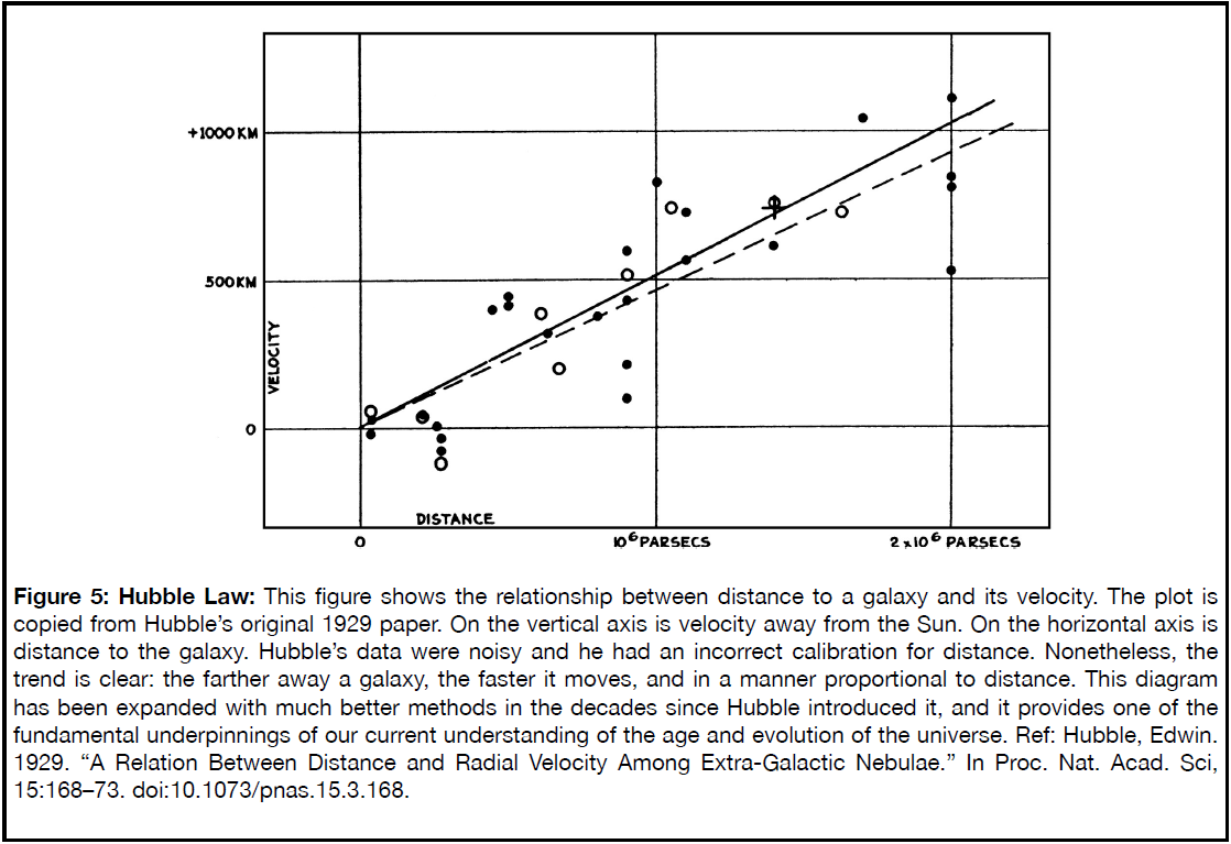
There is a trend of distance with velocity, with more distant objects moving faster. With a nearby exception or two, none of them are moving toward us. The relation is a simple linear one: distance is proportional to velocity. This relation is called the Hubble law.
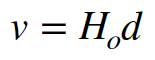
So, what does the Hubble law mean? Hubble’s law shows that recession velocity, `v`, of a galaxy is proportional to its distance, `d`. We may express this relation mathematically as follows, where we write the proportionality constant as `H_o`. It is called the Hubble constant.
That might not be more illuminating than before. But let’s compare it to something that is probably more familiar. We have another mathematical relationship connecting distance and velocity.
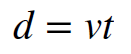
In the equation above, the distance traveled, `d`, is equal to the product of the speed (or velocity), `v`, and the time interval, or the duration of the trip, `t`. It allows us to determine how far we go if we travel at a constant speed for some specific amount of time. So, for example, if we travel at a speed equal to sixty miles per hour for two hours, we will cover a distance equal to 120 miles. Hopefully you are familiar with this equation. We can rearrange Hubble’s law to make it look almost exactly like this distance-velocity-time relation. We only have to divide by the Hubble constant, `H_o`.
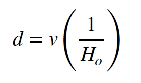
Comparing this equation with the previous one, we see that the Hubble constant is the reciprocal of some time. But what time is that? Well, if we think about it we will realize that, for each galaxy, it is the time required to arrive at its current distance from us, traveling at the speed, `v`, appropriate for that particular galaxy. But note, the time is the same for all galaxies! That is because the closer ones have moved more slowly, whereas the more distant ones have moved faster. At a time equal to the reciprocal of the Hubble constant, all the galaxies were zero distance from us.
So what Hubble’s law is telling us is that all the galaxies in the universe, and therefore all the matter within it, regardless of how far away from us they are at the present time, were all together some finite time ago. Furthermore, if all the matter in the universe was at the same spot at some time in the past, the universe was in a state of extremely high density, pressure and temperature at that time. But when was that?
To answer that question we have to know the value of the Hubble constant. From the Hubble law, we see that it has units of a velocity divided by a distance, or reciprocal time. That is what we expect. But what is its numerical value? That is a question that astronomers have been trying to answer ever since Hubble presented his law in 1929. The best current value is `H_o ≈ 70 km s^-1 Mpc^-1`, meaning that for every megaparsec of distance, a galaxy adds 70 kilometres per second of radial velocity away from us. This value is not yet completely settled (more on that later) but we will use this for the moment.
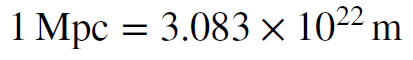
In order to convert this to a time we have to convert the megaparsecs to kilometers, or vice versa. We will do the former. From various references we can find the following conversion.
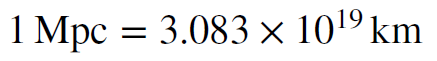
To convert this to kilometers we divide by 1000; a kilometer is one thousand meters, so there must be a thousand fewer kilometers in a Mpc than there are meters. So we have
Now we can use this value to convert the Hubble constant to a time.
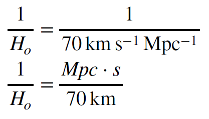
To arrive at this form we moved the terms in the denominator of the denominator into the numerator of the expression on the right. We now substitute the numerical value of megaparsecs, expressed in kilometers.
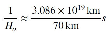
The kilometres cancel out of this equation, leaving only seconds, exactly as we expect. Evaluating the term on the right we have the time corresponding to the reciprocal of the Hubble constant, called the Hubble time.
This is the Hubble time, expressed in seconds. Using the fact that there are about `3.155 x 10^7` seconds in a year, we can express the Hubble time in years.
So the Hubble time is about 14 billion years, give or take. This is the approximate time it has taken for the galaxies to move to their current positions relative to the Milky Way. The expansion rate of the universe (the value of the Hubble constant) is not constant in time. Gravity affects it. Our calculation above does not take this effect into account. Nevertheless, it tells us that at some time around 14 billion years ago, all the galaxies in the universe were together in one extremely dense, hot region. The Hubble time, therefore, is one way to think about the age of the universe. It is, at the very least, related to the age of the universe.
The interpretation of the Hubble time just given is suggestive, but it is not entirely convincing. It was not adopted by astronomers for many years. Before that happened, some of the implications of this idea had to be worked out, and that was not fully accomplished for seven decades.
A Brief Cosmological Aside
Before we turn to the working out of the details of our modern cosmological ideas, we want to make a brief aside. We said earlier that modern cosmology rested on two ideas that came out of the first two or three decades of the 20th century. One was Hubble’s discovery that the universe is expanding, which we have just described. The other idea was general relativity, and we wish now to turn (briefly) to that. It will be in important guide to everything we will discuss later.
The General Theory of Relativity, published by Albert Einstein in 1916, is a theory of gravity. It was not intended to be that when Einstein began. Or perhaps a better statement is that it was not initially understood to be. Einstein had merely (a loaded word, “merely”) wanted to extend his Special Theory of Relativity, which deals solely with constant, unaccelerated motion. He wanted to understand the case of non-zero accelerations. In doing so, he came to understand that there is a close kinship between acceleration and gravity.
Gravity is an acceleration, of course. Usually we think of it as a force, but force is related to acceleration through Newton’s Second Law of Motion. What Einstein found is that there is little to distinguish accelerated motion from gravity. Placed in a windowless box, it is almost impossible for an occupant of that box to make any distinction between accelerating through space or being in the presence of a gravitational field.
This idea, called the equivalence principle, led Einstein to a view of gravity that is very different from the Newtonian idea of a gravitational force. In general relativity, gravity is not a force at all. It is a distortion of space and time (or spacetime) brought about by the presence of mass-energy (which the famous `E = mc^2` from special relativity tells us are not separate, but actually different aspects of the same phenomenon) in the region considered. This distortion of spacetime actually is gravity. (The distortions are often called spacetime curvature, but that nomenclature is misleading unless you happen to know the technical definition of curvature used by mathematicians and physicists. If you don’t, then distortions – as in stretching and compressing – is a more descriptive word.) So just to make this clear, lets repeat: gravity does not cause spacetime distortions, gravity is spacetime distortions.
The mathematical apparatus that describes the curvature of spacetime is too cumbersome and complicated to describe here. We will just point out that it can be used to develop an equation that describes the state of the universe on the largest scales. This equation is called the Friedmann-Robertson-Walker equation, for the scientists who independently derived it using Einstein’s mathematical framework for gravity. The equation does not admit a solution for an infinitely old, static universe, because Einstein’s gravitational equation does not.
Instead, in a non-empty universe, the gravitational equations predict collapse on a fairly rapid timescale. All the mass-energy in the universe attracts all the other mass-energy in the universe. Spacetime basically falls in upon itself. There are ways around this collapse, for instance, if the universe is expanding, but otherwise the equations tell us that the universe should have collapsed. Clearly it has not.
Einstein had realized this, of course. And in the decade or so between the introduction of general relativity and Hubble’s discovery of cosmic expansion, he had worked out a possible solution to this apparent problem. To reconcile his gravitational equation with a static universe he introduced an extra term, one that would counteract the attractive aspects of gravity with a repulsive one. He called this term the cosmological constant. Basically, he introduced an extra term, a “fudge factor” into his equations. It was not an elegant solution. In fact, it had multiple problems, and these were pointed out by other scientists almost immediately. Nonetheless, it was the simplest way to reconcile gravity to a static and infinitely old universe.
Of course, we don’t live in a static infinitely old universe, so Einstein’s “fix” was not required. Our universe is expanding, it is dynamic. When Hubble announced his discovery of that fact, Einstein immediately understood his mistake; he could have used his new theory of gravity to predict a dynamic, expanding universe. But his thinking at that time, like pretty much everyone else’s, was that the universe must be static. There was no evidence to support this belief, it was based only on convention and unsupported bias. In fact, the existence of the universe, when combined with his own theory of gravity, was evidence to the contrary. Einstein later referred to his introduction of the cosmological constant as his “greatest blunder.”
To be fair to Einstein, no one was expecting the results that Hubble found. Not Hubble, not Einstein, not anyone else. The finding of an expanding universe came as a complete shock and forced scientists to fundamentally change their thinking about the universe, its age, its extent and its history. The story of Einstein’s “blunder” is probably best understood as a cautionary tale: don’t become too wedded to convention, be mindful about your biases, be guided by data and reason.
The Big Bang
We have already said that the idea of an expanding universe has certain implications. The first of these has been discussed in the previous chapter: that at some time in the past, all the matter within the universe must have occupied a very small volume. In the Newtonian view of things, we can imagine an explosion of a tiny dense particle that subsequently expands into the surrounding empty space. But this is not the view that is consistent with the general relativistic view of gravitation and spacetime. In general relativity, matter-energy and spacetime have a much more intimate connection. The expansion of the dense, hot material does not move outward into empty space, the expansion is the result of the creation of new space everywhere; it is the newly-formed space between galaxies that causes them to move away from one another. This is a subtle but important difference. According to general relativity, the fabric of spacetime is itself a participant in cosmic expansion, it is not merely a stage upon which the expansion plays out.
Unfortunately, we do not have room to get into all the details of the big bang theory of cosmology. However, we can outline the basic approach. First, we assume that the current conditions in the universe are the result of natural evolution, according to the laws of physics, from that early state to our current one. We can use these physical laws to compute the state of the universe at each moment in its evolution based upon some assumptions about its initial conditions. By comparing the present state of the universe, or the conditions of the universe at some time in the past, we can test our assumptions about the initial state to see if they are consistent with what we observe at a later time, including the present.
We will take a detailed look at two of these observations, that of the relic background radiation from the early universe, and also the abundances of chemical elements we see. Both are intimately related to the conditions that occurred in the early history of the universe.
Before we proceed, there are two fundamental ideas that spring from a relativistic view of cosmology that are worth some of our attention. The first is lookback time. The second is cosmological redshift. We will describe both before moving forward, as they will be useful for understanding what is to come.
Lookback Time
Understanding lookback time is fundamental to understanding modern cosmology. It is related to the finite speed of light. Whenever we look at an object we see it not as it is, but as it was some time ago when the light we see departed from it.
For our day-to-day experience, the time delay is not very important. Only a few nanoseconds are required for light to traverse the distances of familiar objects in our homes, or even outside of them. At 300 million meters per second, light travels about 30 cm in one nanosecond. So in a microsecond, which is a thousand times longer, light travels 300 meters. Clearly, our senses do not allow us to be aware of such tiny time delays in our daily doings with the world.
However, when we look out into space, the finite speed of light does begin to be noticeable. For example, we see Earth’s moon as it was just over a second ago, and the two second delay is clearly discernible in the communications between Earth and Apollo astronauts during the lunar missions. Similarly, we do not see the Sun as it is, but as it was eight minutes ago, the time needed by light to travel across the 149 million kilometers between Earth and the Sun.
In both these examples, the light travel time is still not particularly important. It is still quite small compared to the timescale for either the Moon or Sun to change. As a result, we don’t think much about the time delay inherent in any observation of either body. Such is not the case when we look farther out into space.
The time delay for distant objects in our galaxy can be many thousands, or even hundreds of thousands of years. This is a significant amount of time and can be comparable to evolutionary timescales for many galactic objects. So, for example, some of the nebulae that we can view in the night sky are far enough away that their current state is likely to be markedly different than the configuration in which we see them. In some cases we can watch these objects evolve over a span of decades, and their current state will not be seen by anyone on Earth for thousands of years. But even these timescales are short compared to timescales relevant to cosmology.
When we view objects outside the immediate neighborhood of our galaxy, we are seeing them as they were many millions of years ago, at a minimum. Even the closest galaxy to our own immediate region, called the Andromeda galaxy, is more than 2 million light years away. That means we see it as it was more than two million years ago. In fact, the name of the distance unit, light year, refers to the effect of lookback time. It refers to the distance light can travel in a given amount of time. Light years refers to a distance, not a time, but it does directly convey the amount of time you are looking back over when you view an object: so at a distance of 2 million-plus light years, the Andromeda galaxy is seen as it was more than two million years ago.
Looking farther out into the universe, the finite speed of light has a larger and larger effect on what we see. When we look at most galaxies, we see them not as they are now, nor even as they were a few millions years ago. Most galaxies are so distant that we see them as they were many hundreds of millions – even billions – of years ago; that is the amount of time their light has been traveling, at 300 million km/s, to reach us.
So we would say that we view them at a lookback time of hundreds of millions, or in some cases billions, of years ago. Over such long timescales even galaxies undergo many changes. As a result, we can see the nature of galaxies, and of the universe as a whole, undergo significant evolution when we view objects at different distances, and therefore at different lookback times. Each lookback time provides a snapshot of the universe as it was when the light left those objects long ago.
If we view distant objects as they were far back in the past, can we conclude that those objects are at distances that are the same, as measured in lightyears, as their lookback times? Unfortunately, it isn’t that simple. We have to remember that as the light travels to us, sometimes for many, many millions or billions of years, the universe is constantly expanding. So as the light is speeding on its way toward us, the objects that emitted that light are speeding away from us in the opposite direction. This apparent motion is the result of the expansion of the space between ourselves and the source of the light, and it has an interesting effect on the light as it travels: the expansion stretches the light.
Cosmological Redshift
The amount by which the expansion of the universe stretches light is described by a simple equation, shown below.
The term on the left, `1 + z` is called the expansion factor. It is the amount by which the universe has expanded since the time that the light we observe was emitted at its source. For `z = 1` , the universe has doubled in size, for `z = 2` it has tripled, for `z = 3`it has quadrupled, and so on.
The term on the right compares the wavelength of the light we observe, `lamda`, with the wavelength that the light had when it was emitted, `lamda_0`. From this equation we see that the wavelength increases in direct proportion to the expansion of the universe. If the universe has doubled in size (meaning the distances between galaxies has doubled – we don’t even know if the universe has a measurable “size”), then the wavelength we observe is twice the wavelength the light had when it was emitted.
The factor `z` has a special name. It is called the cosmological redshift, or often just redshift, for short. It describes how much the wavelength of light has been increased, as it traveled from its source to an observer. It happens to all wavelengths, not only the visible ones, but for visible light, a move to longer wavelengths means a move toward the red, hence the name. From gamma-rays to radio, all light has its wavelength increased by an amount described by the cosmological redshift as it travels across the cosmos.
Cosmological redishift is reminiscent of the Doppler shift of a wave, but they are not the same. The Doppler effect is caused by relative motion between the source of a wave and an observer, and so it involves the velocity of one or both of them. Note that there is no velocity in the expression for cosmological redshift. The only thing that matters is the cosmological expansion factor, `1 + z`. This is an important distinction. It happens that many other aspects of the universe are effected by this stretching of spacetime, not only the wavelength of light. Two important examples are the mean density of the universe and its average temperature.
Using our ideas about spacetime and the physics of matter at high densities and pressure, we can imagine what conditions must have been like in the universe at earlier times. We know that the galaxies will have been closer together in the past, and the cosmological redshift tells us exactly how much closer they were. But we can say more than that. For instance, if we consider the material (both matter and light) to be a mixture of gases, then we know that as the universe is taken back to a time of higher densities, the pressure and temperature will both increase. Or conversely, as the universe expands, the material in it will cool, on average, and it will exert less pressure. Both these quantities are also scaled by the redshift relation. By employing the mathematical laws that describe the thermodynamic state of matter, and using the redshift to scale them to different times in the past, we can predict how hot it was and how dense it was. This is the first step.
Cosmic Geometry
We have said that general relativity provides the framework through which we view the history of the universe. It is general relativity that allows us to build testable models of cosmic history and evolution. So it is worth thinking briefly about some of the ideas underlying that framework.
In general relativity, gravity is curvature. By this we mean that gravity is the distortion – stretching and compressing – of space and time as we move from one location to the next. Further, it is mass-energy that creates the distortion.
The mathematics used to describe properties of a curved space, including curved spacetime, is geometry, but not the geometry most of us learned in school. That familiar Euclidean geometry describes a type of flat space, not curved space. In flat spaces, like the top of a table, parallel lines remain parallel forever, they never cross. Additionally, the interior angles in a triangle sum to 180 degrees. You probably learned many other rules of flat spaces that can be described by Euclidean geometry. Incidentally, these rules also describe flat 3-dimensional spaces, not only 2-dimensional ones.
Mathematicians have formal rules to describe a flat space vs. a curved one. We will not bother with those because the mathematics is beyond the level of this work. Basically, though, what we mean by “flat” is that rules similar to (not necessarily identical to) those of Euclidean geometry hold.
Curved geometries are different. Think about the surface of a sphere – like Earth, for example. If you consider parallel lines, perhaps lines of longitude on the equator, you will note that you can trace them north or south to either pole, at which point they all cross. In curved spaces lines do not remain parallel forever.
Similarly, you can imagine yourself taking a journey along the perimeter of a triangle on the Earth’s surface. Start at the equator and walk south until you get to the south pole. Then turn 90 degrees to the right and walk north until you again find yourself at the equator. You will be one fourth of the way around the equator from where you began. Now turn 90 degrees to the right again and walk to your starting point to complete your trip and close the triangle. If you consider the path you have taken and the angles at each point, you will note that they add up to 270 degrees, not 180. This is another way you know that you are walking along a curved space, not a flat one.
The geometrical description of gravity that comes out of general relativity allows us to think in these terms about the universe as a whole. The geometry in the universe, the gravity, is determined by the mass-energy content within it. Some forms of energy tend to make a geometry of one type, some forms of energy make a geometry of another type. In particular, energy that creates attractive gravitational interactions tend to make the curvature similar to that of a sphere. We call that kind of curvature closed because it curves back upon itself and makes a finite, connected surface. Two objects moving parallel in a constant direction in this type of space tend to move closer together over time, sort of like two people starting at Earth’s equator and moving straight south from any two points would slowly approach each other and eventually collide when they reached the south pole. Such curvature is called positive.
Other types of energy create curvature that causes objects to move apart if they start out moving parallel and then move in a constant direction. Rather than having a shape like a sphere, these spaces are more like a saddle. This type of curvature is said to be negative.
We can relate the curvature to more familiar ideas if we think about objects moving under the influence of Earth’s gravity. If you throw an object upward, your keys, perhaps, you cause them to move farther away from Earth. Eventually they stop moving upward and fall back down. By throwing them faster, you can make them go higher, and if you throw them fast enough, they will never come down.
In general relativity we would say that such energy of motion tends to make the geometry of the system open. It contributes negative curvature. On the other hand, the attraction between the object and Earth contributes positive curvature. Generally you cannot throw your keys completely off the Earth because attraction overwhelms the upward motion; the overall geometry is positive and closed.
What if the two contributions are exactly matched?
To answer that question, consider the classical notion of escape velocity. That is the speed at which you must throw an object upward (or launch a rocket, more realistically) in order for it to leave Earth’s gravity and never fall back down. The Apollo rockets to the Moon almost achieved escape velocity, but of course, the Moon is not out of Earth’s gravity (if it was it would not be orbiting Earth), so they were not moving quite that fast.
The escape velocity is the minimal speed for an object to continue to move outward forever, just finally stopping after an infinite amount of time, at least in principle. In general relativity, this transitional case, the one corresponding to the classical escape velocity, is the case of zero curvature. The negative curvature contribution from motion exactly cancels the positive curvature contribution from attraction. The geometry is flat.
Finally, if you throw something a bit faster than escape speed, then even after an infinite amount of time it will have a small residual speed. It never quite stops. The faster above escape velocity you throw it, the more residual speed it has. In this case,
the negative curvature of motion dominates over the positive curvature of attraction, and the overall geometry is negative and open.
So we can think of the geometry of the universe as being caused by a negative curvature contribution from its expansion and a positive curvature contribution from the attraction from all its mass-energy. The overall evolution of the universe in time is determined by the balance of these two. If the curvature is net positive, then the expansion eventually slows, stops and reverses into collapse. If the curvature is net negative, then the universe expands outward forever. All we have to do to determine the fate of the cosmos is find out the amount of each type of curvature and compare them.
With these ideas in mind we are ready to begin to think about modern cosmology the way cosmologists do. Basically, cosmologists have been trying to determine the overall geometry of the universe for decades. The expansion is relatively easy to measure. Hubble’s results were the earliest example of this, and the expansion provides the negative contribution to total curvature. Counting up all the mass in the universe, and thereby measuring the positive contribution, has been harder. Much of the effort in cosmology has been directed along these lines.
Finally, we should mention that there is one other constituent that could contribute to the global curvature, assuming it even exists. That is Einstein’s cosmological constant. It has a repulsive affect, like motion, and tends to cause objects to separate over time. Therefore, it contributes a negative curvature term. For many years it was thought to be negligible. Results over the past two decades have turned that expectation upside down.
Measuring the Universe
It is safe to say that scientists of the early 20th century had never had anything in their lives or careers to prepare them for the disruption that the work of Edwin Hubble was to create. At that time, people’s understanding of the universe was limited to Earth itself. Furthermore, most people, including scientists, thought in terms of timescales that are relevant to human history. Hubble’s work shattered these common notions of space and time. He showed that previous thinking about the cosmos was so far removed from the reality that, we might say, it was not even wrong.
To be fair, scientists at that time did not have a very clear idea of either the size of the universe or its age. The cosmological data, to the extent that any existed at all, was
extremely crude. Without data it is not possible for scientific progress to occur, nor can we make informed judegments about which of several competing theories might be correct, and which of them wrong.
However, even early on there was very basic observational data readily at hand, even if
not always appreciated. An argument first put forward by Heinrich Wilhelm Olber in the first part of the 19th century (and then by others in more detail subsequently), suggested that the universe could not be both infinitely old and infinite in extent. If the universe were infinitely old and contained an infinite number of stars spread more or less evenly throughout, then, so the argument went, the night sky could not be dark. Instead, no matter what direction one looked, the line of sight would intercept the surface of a star. The sky should be as bright as the surface of the Sun. Clearly, this is not what we observe.
From the reasoning of Olber, often referred to as Olber’s Paradox, the universe could not be both infinitely old and infinitely large, but it could be one or the other. Or neither. Without any data to decide one way or another, astronomers debated back and forth, but there was no way to resolve the issue.
In 1920, Harlow Shapley reported the first results to begin to settle the argument. Shapley used the system of globular star clusters to locate the direction and distance to the center of the Milky Way. Astronomers were astounded. Few had imagined, or could have imagined, how large our galaxy was.
Shapley found that the distribution of globular clusters was centered on a point in the
constellation Sagittarius, and located nearly ten thousand parsecs (30 thousand light years) from Earth. Since this distribution of massive star clusters was centered on that point, it seemed reasonable to assume that the center of our galaxy must be there, too. That in turn meant that our galaxy is many tens of thousands of parsecs across, or about 100,000 light years from edge to edge. Surely, some argued (Shapley included), an object so huge must contain all that there is in the universe. But additional evidence was soon to show that even the immense size of the Milky Way did not account for all of the observable universe.
The Primordial Background Radiation
Once we have an idea of the temperature and density in the universe, we can begin to use the laws of physics to predict what sorts of interactions the matter and light will undergo. For example, in a hot gas we know that atoms undergo violent collisions that can excite their electrons. When the electrons de-excite, they emit photons, filling the surrounding space with light. This light will further interact with the atoms, and if the interactions are frequent enough, the matter and the light will be in thermal equilibrium, meaning they can both be characterized by a common, single temperature.
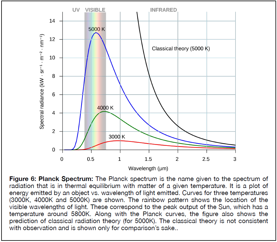
When matter and light are in thermal equilibrium, we know the light will have a particular kind of spectrum, a spread of brightness (or number of photons) with energy (expressed as either frequency or wavelength). This spectrum is called a Planck spectrum, after the German physicist Max Planck who in 1900 was the first to devise a theoretical explanation for it. The spectrum of Planck radiation is shown in Figure 6 for several different temperatures. It has the appearance of a skewed bell curve.
Planck curves describe radiation that is in equilibrium with matter. That means that the matter and the radiation interact often enough that their characteristic energies are the same. Clearly that is not the case in the universe today, where radiation can stream billions of light years (so for billions of years) without ever interacting with matter. But the universe was not always that way.
There was a time in the early universe when the matter density was so high that radiation and matter interacted with one another frequently enough to keep the two in equilibrium. The radiation at that time would have had a Planck spectrum as a result. As the universe expanded, the density dropped. Eventually the density would have reached a state where interactions between photons and atoms could no longer maintain a common temperature. The matter would have continued to sustain collisions with itself, but the radiation would have decoupled from it. From then on the photons would have streamed across the universe, unperturbed by the matter.
The relic radiation from this time should still be present, and it should still reflect the Planck nature it carried back then. The only difference is that the wavelength of all the photons would have been stretched by an amount equal to the amount of expansion since that time due to the cosmological redshift. We therefore have a powerful and important prediction of this theory of cosmic origins. It is so important that we will state out separately.
Prediction One: The universe should be filled with a relic radiation of an early hot phase that reflects a period when matter and light were in thermal equilibrium. This relic radiation will have a Planck spectrum, but now of a temperature cooler by a factor of 1 + z, dictated by the amount of expansion that has taken place since it was last in thermal equilibrium with matter. The radiation should be everywhere. It should have a constant spectrum and will now reflect a temperature of a few kelvins, the cosmic expansion having dropped it from its original few thousand kelvin.
The details of the predicted background radiation were developed by a team of scientists at Princeton University, in New Jersey. By the 1950s they had devised not only the expected properties of the radiation, but they had also designed an experiment they hoped to use to detect it. However, their hopes were dashed by two researchers at the Bell Labs facility of AT&T.
Until the middle of the century, telephone calls had been carried by cables strung across town, continents and seas. But a new technology was beckoning. It used microwaves to transmit the telephone signals. It had the advantage of not requiring the laying of cables, but some technical barriers had to be overcome before the technology could be deployed. Among these were sources of noise that interfered with the microwave signals.
As part of its microwave telecommunication program, AT&T hired two radio astronomers to track down sources of radio noise associated with celestial sources. These astronomers used a radio horn to scan the skies, making a catalog of sources that would have to be screened from any telecommunication system. Many sources were found, but after the discrete sources had been accounted for, there remained a signal that seemed to be coming from every direction. No matter how the scientists tried to account for it, no source was found. They even looked for sources internal to their equipment, double checking that bad electrical connections or imperfections in their radio telescope were not creating the signal. Nothing worked. They were at a loss to understand the origin of the noise.
As luck would have it, one of them received a copy of a paper from a friend in the physics department at MIT. The paper, still in preparation, was by the Princeton group. It described the properties of the radiation field they expected to see as a remnant of the hot and dense early phase of the universe. As the Bell Labs astronomer read through the paper he realized what the unidentified source was in his and his colleague’s measurements: they had detected the cosmic background.
The Princeton group had predicted a uniform radio signal seen in every direction in the sky. It’s expected temperature (the temperature corresponding to its Planck spectrum) would be a few kelvin, meaning it would peak in the microwave region of the
electromagnetic spectrum. The signal seen by at Bell Labs was exaclty that, uniform around the sky with a temperature of `3K`.
At the invitation of the Bell Labs researchers, the two groups met at The Labs to look at the antenna and discuss the discovery. They decided to publish their results simultaneously. The Princeton paper would describe the theoretical prediction and the Bell Labs team would report their discovery. Both papers appeared, back to back, in the Astrophysical Journal Letters in 1965.
This discovery was the first to confirm a prediction of what had come to be known as the big bang theory, the proposal that the universe had started in a state of very high temperature and density and that, for unknown reasons, it had expanded and cooled from that initial state. Because the Planck curve of the background radiation peaks in 3K the microwave part of the electromagnetic spectrum, it is often referred to as the cosmic microwave background, or CMB.
Detecting the background radiation was only the beginning. Once it had been seen, scientists set about trying to test other aspects of the theory. In particular, the spectral shape of the radiation was predicted to be have a Planck spectrum to high precision. The observations at Bell Labs were consistent with a Planck curve, but they might have had any other shape as well. They were made at only a single frequency band, and that is not sufficient to determine the spectral shape. Verifying the spectral prediction required purpose-designed experiment, one that could measure the intensity over many different frequencies, and thus determine the spectral shape to high precision.
Over the following decades, scientists found other properties of the CMB that were of interest. During the 1970s and 1980s they had learned that matter in the universe is clumped. Galaxies are not randomly distributed in space, they are collected into large filamentary structures and groups. In between the groups of galaxies are voids where no galaxies are found. The microwave background should reflect these density fluctuations on smaller angular scales than could have been measured using the telescope at Bell Labs.
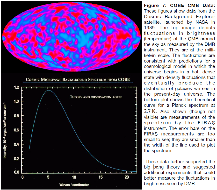
In order to precisely measure the CMB spectrum, and to look for the small temperature fluctuations that would reveal the seeds of what came to be called the large-scale structure of matter, a satellite called the Cosmic Background Explorer (COBE, for short) was launched by NASA in 1989. The satellite carried three instruments, each made by a different group of scientists. Two of the three were designed to pick out different aspects of the CMB.
One group, located at NASA’s Goddard Space Flight Center, built an instrument called the Far InfraRed Absolute Spectrometer, or FIRAS, designed to measure the shape of the spectral energy distribution of the CMB. Another group, at the Lawerence Berkeley National Laboratory on the campus of the University of California, Berkeley, built an instrument called the Differential Microwave Radiometer, or DMR. This instrument was built to measure small fluctuations in the brightness of the radiation, corresponding to the seeds of structure.
COBE was spectacularly successful. It was able to show that the CMB was, to the ability of the spacecraft to measure, consistent with a perfect Planck spectrum, having a temperature of 2.7K.In addition, COBE measured small fluctuations in the temperature that were consistent with the large scale structure we see in the universe. The angular resolution of COBE was not good enough to measure the details of the fluctuations, but it was sufficient to show that the CMB was completely consistent with the predictions of the big bang theory. The data from the COBE satellite are shown in Figure 7.
The success of COBE was compelling and gratifying. It suggested that cosmologists were on the right track. However, it also suggested that more was possible. If, as seemed to be the case, the universe began in a hot dense state that gradually expanded and cooled to form the galaxies we see today, then there was more information in the CMB than had hitherto been seen. To understand why this is the case, we have to think about the connection between the universe we see today and the universe from which it emerged.
The universe today is clumpy on small scales. We see galaxies clumped into groups and clumped into long filaments. On the very largest scales the universe is quite smooth, it is not clumped. It is only on smaller scales (but still much larger than single galaxies) that the clumpiness becomes apparent. And the structures that we see have been enhanced by gravity over the roughly 14 billion years since the cosmic expansion began. On small scales, the galaxies themselves contain clumps of stars and nebulae, of course, but those don’t concern us here.
If we look at the largest scales at which clumping is visible, we should see a correspondence with fluctuations in the CMB. Why is this? Because the CMB is not a picture of the universe now, it is a picture of how the universe looked more than 13 billion years ago, when the CMB was formed.
Recall that, back then, matter and radiation were in equilibrium. They were coupled. The high density and temperature caused photons interacted strongly with the electrons and nuclei that existed. The interactions were so strong that the radiation prevented the matter from combining to form atoms, and certainly from collapsing via gravity into large objects like stars or galaxies.
Eventually, as the expansion cooled the universe, the temperature and density dropped
enough that collisions between matter and photons were no longer frequent. At that point, the electrons and atomic nuclei could combine and, for the first time in the history of the universe, form atoms. The photons were then able to travel vast distances without ever interacting directly with matter, creating the CMB that we see now. Of course, the matter was also free of interference from the photons, and it could begin to collapse.
However, the matter was not spread uniformly in the cosmos then, just as it is not now. As the matter became free to collapse, the collapse would begin first and proceed faster in areas where the density was, for whatever reason, slightly higher than average. It would start more slowly in areas where the density was not as high. As a result, there should be a spectrum of structures that we see in the universe now that corresponds to the spectrum of density fluctuations that were present in the early universe.
Photons streaming across these areas of collapse would have their energies altered slightly. They would gain energy (get hotter) as they fell into the dense regions, and then loose energy as they climbed out the other side. These effects would be asymmetric though, because in the time required for the light to cross the collapsing regions the density of the regions could grow appreciably. As a result, the photon energy loss would be greater than the photon energy gain, and high density regions would have the net effect of making cool spots in the CMB. The hotter regions in the CMB would correspond to the lower density regions in voids.
The bottom line is that the cosmic microwave radiation should reflect the clumping of matter at early times. The high and low density regions that now correspond to clusters and voids should be related to high and low temperature fluctuations in the cosmic background radiation.
We don’t mean that we should be able to make a one-to-one correspondences between a particular galaxy cluster and a particular fluctuation in the CMB: the CMB is seen at a different time and place in the universe than any galaxy or galaxy cluster. What we should see, however, is the same spectrum of fluctuations. Galaxies/clusters and CMB fluctuations should match in a statistical sense because the average conditions were the same everywhere in the universe. This is what the COBE results demonstrated.
COBE did not have the ability to measure the full spectrum of the CMB fluctuations. It was designed only to look for the presence of fluctuations at a certain size and temperature level, not study the fluctuations in detail. By the late 1990s and early 2000s, scientists were ready to test their predictions about the CMB fluctuations in a more detailed way. They had built, or were building, an array of experiments designed to look a the full fluctuation spectrum of the CMB radiation around the sky.
The first of these experiments were flown as balloon payloads. The balloons carried the experiments into the upper atmosphere, beyond the regions where absorption would have a pronounced affect on the observations. At these altitudes, the experiments had an unobstructed view of the sky and could make careful measurements of the CMB.
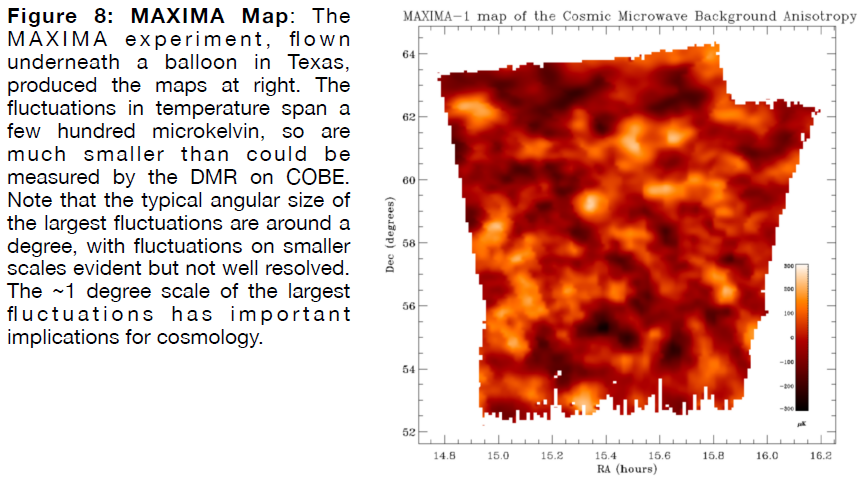
Two of these CMB experiments were flown in the late 1990s. The Millimeter Anisotropy Experiment Imaging Array, or MAXIMA, was built by a team in Berkeley and flown underneath a balloon launched near Palestine, TX at an altitude in excess of 130,000 feet. The experiment had limited angular resolution, so it could only determine the largest-scale peaks of the CMB spectrum. Nonetheless, it did measure the size of the largest and strongest peak during its two flights in 1998 and 1999. Its eight hours of data provided the maps shown in Figure 8, and culminated in the first major breakthrough in finding the shape of the CMB spectrum.
A completing experiment to MAXIMA was called BOOMERANG, for Balloon Observations of Millimetric Extragalactic Radiation and Geophysics. It was built by an
international team with leads at CalTech and at the University of Rome, in Italy. BOOMERANG worked along similar design to MAXIMA. In fact, the two teams had been one, but split. Both were balloon-borne missions, but unlike MAXIMA, BOOMERANG was launched in Antarctica, not in the USA.
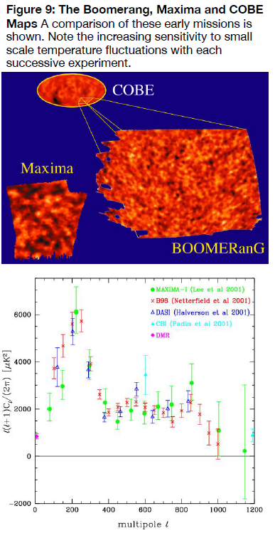
The primary science flights of BOOMERANG occurred in 1998 and 2003. The payload was launched from the McMurdo Station, and it flew in the circum-antarctic high altitude winds (the polar vortex), which carried it completely around the periphery of the continent. That was what gave the mission its name – and its somewhat cumbersome acronym. The entire trip around the edge of Antarctica required about ten days, and this allowed the payload to observe for a much longer time than MAXIMA had. It thus obtained more detailed data. The fluctuation maps from BOOMERANG are shown in Figure 9. For comparison, maps from MAXIMA and COBE are also shown. You can see the better angular resolution attained from COBE to MAXIMA to BOOMERANG.
Viewing the sky maps from these
missions is instructive, but it is not the best way to understand the information they contain. A more mathematically rigorous and sensitive technique is used, called a Fourier transform. The details of this
procedure are not important here. We only need to know that a plot of the
Fourier transform shows how much of the fluctuations in the sky occur at
various angular scales. If the strongest fluctuations occur at large angular sizes, then the Fourier transform of the maps will have a large amplitude for these sizes. If the strongest fluctuations happen at small angular scales, then the Fourier transform will be higher at small scales. The plot of the Fourier transform for the BOOMERANG and MAXIMA data are shown above. Results from several other experiments (which we have not
mentioned) are also plotted.
The units used to plot these results are quite abstract and not worth delving into here. All we need to know is that the vertical scale measures the power of the fluctuations in an appropriate (if obscure) unit. Likewise, the horizontal axis is the angular scale measured in another strange unit denoted as `l`. It is enough to note that the peak of the spectrum occurs at a multipole value `l~~200`, which corresponds to an angular size in the sky of about 1 degree. So what does this mean? The biggest prize is related to the biggest peak: it indicates the overall global geometry of the universe, and it says it is flat. Expansion energy matches attraction exactly. More on this below.
The balloon-bourn CMB experiments were the first to measure the largest features of the fluctuation spectrum, and they measured the cosmic geometry. However, they lacked the resolution and sensitivity to see smaller features. To do that, satellites were needed. Fortunately, these had been in the works and were ready to take up the study of the CMB shortly after the balloon experiments.
Between 2000 to 2010 two CMB satellites were launched. The first of these, launched by NASA in 2001, was called the Wilkinson Microwave Anisotropy Probe, or WMAP. The second, launched by the European Space Agency (ESA) in 2009, was called Planck. Both were able to measure fluctuations on a smaller angular scale than the balloon experiments could. These fluctuations are related to detailed aspects of big bang cosmology, and they allow a more thorough testing of the theory than earlier observations.
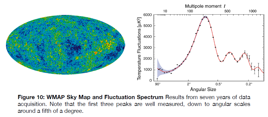
The sky map and derived spectrum of fluctuations from WMAP is shown in Figure 10. Note that the data are much more sensitive than those obtained from balloon the missions. This is because WMAP, unlike its Earth-atmosphere based predecessors, could stare continuously at the sky, building up signal over a comparatively much longer time. The data shown are for seven years of data, a timespan the could never be achieved from a balloon payload experiment.
Sensitivity increased again with the deployment of the Planck satellite, as is shown by the sky map and derived plot of its fluctuation spectrum in Figure 11. This increased sensitivity provided high precision measurements of several key predictions of the big bang theory.
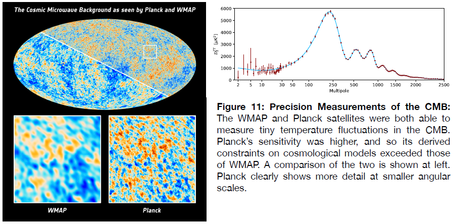
In the spectrum above, there are three clear peaks visible, plus several minor ones on
the far right. The prominence of these peaks and their position along the horizontal axis
depend strongly on conditions in the early universe. In particular, they depend upon the
kinds and amounts of the materials contained in the universe.
We cannot go into detail on how the peaks are produced, but we will describe the meaning behind the three most prominent ones.
- The First Peak: The size and position of the first peak (the left-most one) is determined by the overall geometry of the universe, as we mentioned earlier. The peak was first measured by balloon experiments, and the satellites greatly increased the precision of those measurements. From this peak we know that the global geometry is flat, which is to say that the energy in expansion is closely matched to the energy of gravitational attraction. We also know that the matter content is around 30% of the total energy of the universe.
- The Second Peak: The position of this peak, and its prominence relative to the third peak, is sensitive to the baryon content in the universe. This is distinct from the total matter content; baryons are matter composed of quarks, i.e., normal atoms. The second (and third) peak suggests that about 5% of the total energy is in baryons, or one sixth of the matter, leaving an additional five sixths in a form that is not known and is referred to as dark matter, a result also consistent with observations of galaxies and galaxy clusters.
- The Third Peak: The position of this peak is sensitive to the amount of dark energy in the universe. This energy is possibly the cosmological constant first postulated, and later retracted, by Einstein. From the position of the third peak we can infer that the dark energy comprises 70% of the energy content of the universe. Together with the first peak, it means that 30% of the energy is composed of matter, both baryons and dark matter.
There is additional information that can be extracted from the CMB, but these are the most interesting findings. The Hubble parameter can also be extracted, and the most
current CMB measurements, from the Planck satellite, give a value of `H_0 = 67.37 +- 0.54 km s^-1 Mpc^-1`. This is at odds with other measurements, and that is discussed in the Structure and Composition of the Universe section.
See the Additional Resources tab on the left.
The Dark Matter and Large Scale Structure
To conclude this discussion of the CMB we should consider for a moment the implications of the dark matter. Strong evidence for its existence was known long before the CMB fluctuations were measured. This evidence is related to galaxies and large-scale structure, which is discussed in the Structure and Composition of the Universe section of this site. Much like other evidence, the CMB evidence is indirect: it shows the effects of the dark matter, but it doesn’t say anything in particular about what it is. Furthermore, it shows that the dark matter had already imprinted the seeds of structures on the universe only a few hundred thousand years after the big bang. This is quite interesting, because the baryons alone would not have been able to create these structures in such a short time. Recall that the features in the CMB are the result of the matter – the normal matter – interacting with the photons. The dark matter cannot do this because it does not interact with light at all.
Be that as it may, the CMB clearly shows the presence of large density variations in the
universe at a time when matter was not able to create those concentrations. Only a type of matter that does not interact with light could have. In fact, without something like dark matter to seed these regions of enhanced density, there would not have been time for the structures that we see today to grow at all. So the presence of dark matter is suggested not only by the overall geometry of the universe, but also by the fact that we see galaxies and clusters of galaxies. Without dark matter to trigger the formation of structure at very early times, even earlier than the creation of the CMB, there would be no structures like the ones we see now in the universe.
The Production of Light Atoms
The existence of a relic background radiation is not the only implication of an early hot
dense phase in the universe. If we imagine what conditions were like even before this radiation was created, we know that the density and temperature would have been higher still at earlier times. We can then ask what effect these earlier times would have had on the universe today. In particular, conditions at that time would have produced the basic basic building blocks of matter that exist now.
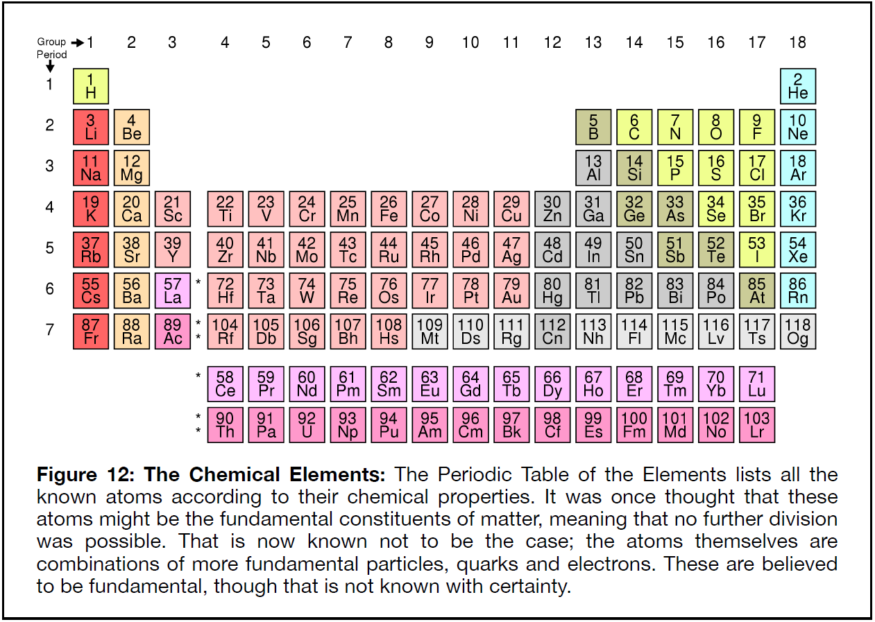
You probably know that all matter in the universe is made of combinations of 92 different kinds of atoms. These atoms are often displayed in The Periodic Table of the Elements, first laid out by the Russian chemist Dmitri Mendeleev in the 19th century. The Periodic Table is organized according the the chemical properties of the atoms, that is, according to which atoms are likely to form chemical compounds with which other atoms. A version of the Periodic Table is shown in Figure 12.
At the time the Periodic Table was created, scientists did not understand the nature of
matter. They did not know that atoms are the fundamental unit of the chemical elements. That knowledge had to wait until the opening decades of the 20th century. Since then, we have learned that even the atoms are not fundamental. They are made of even smaller particles, the quarks and leptons. Two different kinds of quarks combine – in groups of three – to form protons and neutrons, the particles that make up atomic nuclei. The electrons, which are a type of lepton, combine with the nuclei to form atoms.
Our understanding of the processes by which atoms are created by combinations of more fundamental particles increased vastly over the decades of the 20th century. Eventually, it reached a point where we could use this understanding to predict how conditions in the early universe, where temperatures and densities were unimaginably high, would have affected the forms of matter we see today.
If we back up the clock far enough, we come to conditions that are too hot for atoms
to exist. Under those conditions, the motions of particles are so energetic that the electrons and nuclei cannot form stable atoms. Collisions blast them apart as quickly as they are created. Instead, the nuclei and electrons exist independently in a hot ionized gas called a plasma. It was under these conditions that the background radiation was created.
Earlier still, under yet denser and hotter conditions, even the nuclei would have been unstable. Collisions between them would have prevented them from forming any heavy nuclei, such as we see in most atoms in the Periodic Table. Instead, there would not have been anything heavier than hydrogen and helium, and perhaps some lithium.
And before that? The temperatures and densities increase as we go to earlier and earlier times. Eventually they reach a point where the nuclei, too, become unstable. They break apart into their constituent quarks, as well as other fundamental subnuclear particles, including the gluons by which quarks interact with each other.
We have theories that can predict how much of the physics would have played out at
these early times. Our theories describe how three of the four known interactions of matter came into being, including the two nuclear interactions (called the strong interaction and the weak interaction) and the electromagnetic interaction. Only gravity is left out. Some theoretical predictions can be well-tested because they make robust projections about observable effects in the present-day universe. Others are more speculative because we have not yet worked out our understanding of the relevant physics. We will take up the well understood phenomena first, and then provide a brief overview of what remains to be done.
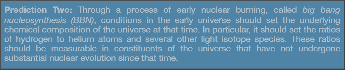
One of the best understood predictions to come out of the Big Bang Theory is in the
distribution of the light atoms, up to around lithium. This is because the physics of nuclear reactions is well known; we can recreate those conditions in the laboratory, and they are used in both nuclear power reactors and in nuclear weapons. So, what do these predictions foretell? The basics are stated in the box below./p>
Imagine a time in the universe when it is still too hot for nucleons (protons and neutrons) to form. Whenever quarks come together to form a nucleon, collisions break them apart again. These collisions can take place with quarks, with electrons, with photons or with other particles that are created in those conditions. Matter at this time is a mixture of quarks and leptons, with accompanying photons and gluons.
As the universe expands, its temperature and density drop relentlessly. Eventually, cooler temperatures are reached, meaning that the collisions become less violent, less prone to break apart any nucleons that have formed. Decreasing density means that collisions are less frequent, so any nucleons that do form are more likely to survive over time. During this phase in the history of the universe, the quarks and gluons become bound into nucleons, and matter is composed of a mixture of baryons (protons (`p`), neutrons (`n`), electrons (`e^-`), positrons (`e^+`), neutrinos (`v`), antineutrinos (`bar v`) and photons (`y`). The high temperature (around `10^10`K) means that these particles will be kept in thermal equilibrium via the equation network shown below.
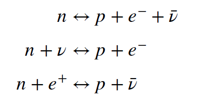
This reaction network sets the ratio of neutrons to protons. At higher temperatures it is
relatively easier to make neutrons, so the ratio is higher. As the temperature drops, the number of neutrons relative to protons also drops. Eventually, the temperature is low enough (but still tens of millions of kelvin) that neutrons are not produced at all. That is the point at which it is possible to begin to combine nucleons into heavier nuclei through a process called nucleosynthesis.
From basic nuclear physics we know that the state of matter at the beginning of this
nucleosynthesis epoch would have had protons about seven times more abundant than neutrons. Collisions between the two would have quickly consumed all of the neutrons (those that didn’t decay first) to produce alpha particles. These would, in time, become nuclei for the most common type of helium. We can understand this graphically using the schematic in Figure 13.
An `a` particle is a combination of two protons and two neutrons, as shown in the boxed area on the left side of the diagram. For each of the two neutrons in the particle there is one accompanying proton and six other protons that are not incorporated into the`a` particle. The free protons are thus single particles by the time all the neutrons have been used up. This tells us that, after all the neutrons have been combined into alpha particles, there will be a dozen protons left over.
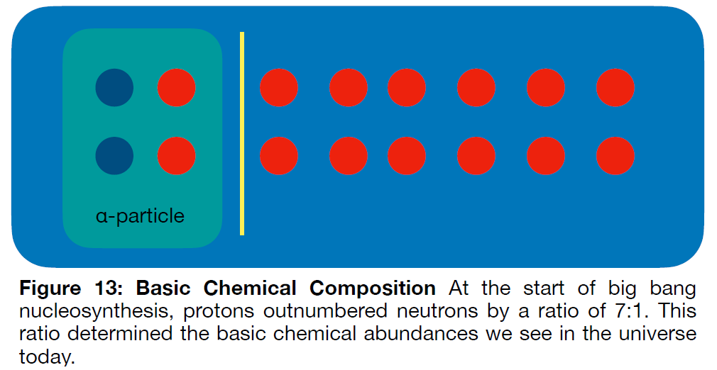
The process of producing alpha particles is halted by the exhaustion of the neutron
supply, and thereafter the ratio of ’s to protons is fixed. As a result, we should see the imprint of this early time in the universe on its present-day chemical composition.
The `a` particles eventually, after the temperature drops sufficiently, combine with two
electrons to form helium atoms. The protons combine with single electrons to form hydrogen atoms. So we should see that there are twelve hydrogen atoms in the universe for each helium nucleus.
This ratio is sometimes stated in terms of mass, not number of atoms. Since each `a` particle is four times heavier than a proton, and since they should exist in the ration 1 `a` to 12 protons, we should see that helium atoms comprise 25% of the mass in the universe, and hydrogen atoms comprise 75%. And they do.
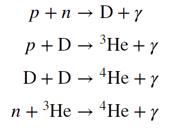
The process outlined above is slightly oversimplified, as you might suspect. The process by which protons are converted into `a` particles is a multistep one. Some of the intermediate nuclei produced should also be left over. These include the mass-three isotope of helium (two protons and one neutron) and the mass-two isotope of hydrogen, called deuterium (`D`), which has a proton and a neutron. There are also small amounts of other light elements produced, like lithium, for example. Some (not all) of the nuclear reactions that occur during this time are shown below.
The amount of each element that is produced depends sensitively on the details of the physical conditions at the epoch of nucleosynthesis. Unlike the simple relationship between helium and hydrogen, the production of other light elements is too complicated to be easily described here. However, it can be modeled and then calculated via systems of coupled equations that represent the thermodynamic state of the universe, the amount of matter and radiation it contains, and the details of the nuclear reactions that produce heavier nuclei from light ones. This has been done, and the the results are summarized in Figure 14.
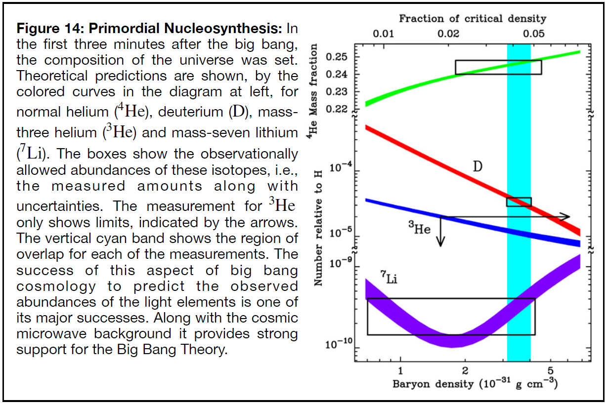
You might notice that lithium is the heaviest element shown. That is due to the short time for primordial nucleosynthesis; it only lasts about three minutes. The rapid expansion of the universe and the resulting decrease in temperature and density halt heavy element formation after this time. It is not until stars form, many millions of years later, that the process is again possible.
Nucleosynthesis is further hindered by the lack of strongly bound stable nuclei with
either 4 or 5 protons (beryllium and boron) to act as steps to building heavier nuclei. The gap presents a barrier to the formation of the elements beyond lithium. Stars are able to surmount this barrier only because they have millions – even billions – of years in which to do so. During primordial nucleosynthesis the time is simply too short and the density too low.
Finally, you might protest that, if helium is 25% of the mass of all atoms, and hydrogen
is 75%, that leaves 0% for everything else! You are not wrong. But if you look at the diagram above, the abundances of the atoms beyond hydrogen and helium are minuscule. `overset3` `H` is below a few parts in `10^5`. Lithium is rarer still, less than a few parts in a billion. And this remains true even after 13 billion years of heavy element formation in stars: the vast majority of atoms in the universe are either hydrogen or helium. All the other atoms combined make up only a few percent by mass, or a few percent of a few percent of a few percent by number.
Inflation
You might have noticed that everything we have described occurred after the universe was a few minutes old. The nuclear reactions of big bang nucleosynthesis commenced around a minute after the big bang and were completed by around three minutes. That was the brief period in which the density and temperature made nuclear reactions possible. The cosmic microwave background was created nearly 400,000 years after the big bang, when the density and temperature of the universe had dropped enough to allow the photons to decouple from the matter and stream undisturbed across the universe. Over the roughly 14 billion years since that time, the structures of galaxies have been forming and evolving, as is described in the Structure and Composition of the Universe section. The conditions in the early universe that we have discussed set up the initial conditions from which all these processes could spring… But what set up the initial conditions for what came before that?
To answer that question, we have to delve, briefly, into the idea of Cosmic Inflation, or just inflation, for short. Inflation is an idea that originated in the late 1970s and early 1980s. It was independently developed by scientists in the United States and the Soviet Union, and it has undergone substantial development by many others since then.
Inflation was first developed as a way to explain an aspect of electromagnetic theory and particle physics, namely, the absence of any magnetic analogue to electrons and protons: there are no observed “magnetic charges.” People quickly understood that the theory made some interesting predictions about the universe on large scales, and that some of these were born out. So, what is inflation, and what are it’s predictions?
Simply put, inflation is the idea that the universe underwent an extremely high rate of expansion over a very short period early in its history. Specifically, in a time after the big bang between` ~ 10^-36` and ` ~ 10^-32` seconds, the size of the universe is postulated to have increased by, at a minimum, a factor of ` ~ 10^20`. To drive the point home, if you were standing talking with someone, separated by a distance of a meter before inflation, an instant later (` ~ 10^-32 s` ), that person would be (at least) `10^20` away. That is more than 10 million light years! Inflation expanded space (inflated it, hence the name), and this carried objects in that space away from each other at an astounding rate.
Note that this does not violate any speed limit imposed by the speed of light and relativity. That
is only relevant to objects moving through space. Inflation expanded space itself, and any objects were simply along for the ride. They never moved through space at all.
This sounds like a fairly preposterous idea. Why do many cosmologists think it might be true?
To understand why, we have to look at some of the theory’s predictions and how they solve certain troubling aspects of Big Bang Cosmology.
The Puzzle of Isotropy and Homogeneity
The standard big bang model has several puzzling aspects. One of them is the observed fact that the universe appears to be (on average) remarkably the same everywhere. The average density is roughly constant, and the average temperature is the same everywhere, as was shown by COBE. How can this be? Or, you might be asking yourself, why is this puzzling?
If we think through the implications of making two measurements of the CMB in opposite directions in the sky, we immediately run into a puzzling situation. The light we see, from each of the two directions, was emitted shortly after the big bang. It’s lookback time goes all the way back to about 400,000 years after the big bang. Since then, it has been traveling toward. That means that the two regions we view have never been able to see each other or interact in any way. There has only been time enough in the history of the universe for the light to travel half the distance between them – to us! Any light reaching us from all the way to our left has not had time to reach the region we are seeing at the same lookback time all the way to our right, and vice versa. How do they know to have the same temperature and the same density? This is a problem no matter which two directions we look, so long as they are directly opposite to one another in the sky.
Of course, it is possible that it is merely coincidental that the entire universe is the same everywhere. However, in an event that would have presumably been as violent as the big bang, it seems incredible that such would be the case for any two oppositely directed locations in the sky. Instead, it begs for an explanation.
The Puzzle of Geometry
The second puzzling aspect of the standard big bang is the geometry of the universe, which is very nearly flat. We have already discussed how the geometry is a balance between the negative curvature terms of the expansion and the positive curvature terms of the mass-energy content in the universe. For decades these were known to be a match to a very high degree, at least to around a factor of around 2 of each other. Again, it was puzzling. Why should they be so closely matched, but not exactly matched?
Of course, if they were far out of balance, then the question would be moot. In such a
universe there would be no cosmologists to ask it. A universe in which matter is highly dominant would have collapsed under its own weight long ago. A universe in which expansion was highly dominant would have expanded so fast that no structures could have formed. And no cosmologists, either.
But we don’t live in either of those universes. We live in one in which the two are close enough to being in balance that there are cosmologists to sit around and ponder the questions surrounding the existence of galaxies – and cosmologists! Again, the situation begs for an explanation.
The Puzzle of Structure
Finally, cosmologists have wondered why there are structures in the universe. The seeds of these structures had to be set in place at early times so that they could grow into the massive systems we see now. How did that happen, and why? This question is not as compelling as the first two, but still, one wonders.
Inflation To the Rescue
It turns out that inflation can naturally explain all of these puzzles. Let’s take each of them in turn.
First, inflation can explain the isotropy (all directions being the same) and homogeneity (all locations being the same) puzzle. If the universe was much smaller at very early times, then there would have been a chance for any temperature differences, as well as large differences in density, to smooth out. Then, the rapid expansion during inflation would have caused these locally equilibrated volumes to expand to an immense size; recall that a volume a meter in size would have expanded to one `10^20 m` across, at a
minimum. Then that region would have continued to expand according to the Hubble law to an even bigger size over the age of the universe. So what we see now, residing inside one of these immense regions, is that everything is at the same temperature. If there are neighboring regions with different conditions, we cannot see them. The universe is not yet old enough for light to have traveled the vast distances between us and them.
Inflation Solves the Flatness Problem
Inflation answers the geometry puzzle in a similar way. Imagine that the universe has some
global curvature that is either positive or negative. Then expand the universe by a factor of
`10^20`. Globally, the geometry of the universe has not changed, but inflation has made “globally” somewhat moot. We only see the region very (relatively) nearby, and that necessarily looks flat. This can be understood by considering a familiar curved object, maybe a ping pong ball. It has a size of an inch or two. Now imagine blowing it up to the size of Earth. Clearly, if you are standing on its surface, it will appear flat, just as Earth does. And that is an increase of only a factor of around `10^8`. The inflationary epoch we are discussing was vastly greater. Of course, if you go off the surface of the ping pong ball sufficiently far, you will be able to see its curvature. But we cannot go outside our local area of the universe. We can barely get off Earth. So our universe looks flat, no matter where you are inside of it.
Inflation Solves the Structure Problem
Finally, inflation also has an explanation for the seeds of structure. At the time of inflation, the universe was much, much smaller than it is now. Everything was packed into a volume so small that the average density and temperature were nothing that we can begin to imagine. We can, however, use the known laws of physics to guide our thinking. Under those conditions there would be what we would consider chaos, with violent shifts in density and pressure. Particles would have been created and then annihilated constantly. This would have naturally lead to differences in density over a vast range of scales. When inflation happened, any density
enhancements would have been frozen in place and inflated with the rest of spacetime. So would areas with lower density. Then, as the universe continued to expand, the density enhancements would have grown as gravity attracted material into them. The areas of low density would also have become more pronounced as the sparse material they contained drained into the high-density regions.
At first this would have only been the dark matter. The normal matter would have been prevented from collecting into these regions by the photons and high temperatures. But then, once the temperatures had dropped and matter and light were free of each other’s grasp, the normal matter, too, began to collect into high density regions, eventually forming the galaxies and galaxy clusters we see in the universe today. At the same time, the photons would have begun their journey across the universe, forming the background radiation.
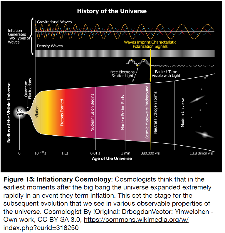
Inflation is still a conjectural idea. It does make predictions (several outlined above) that have been borne out. However, its details remain to be understood. There are several different forms that inflation could have taken, and there are different ideas for what initiated it in the first
place.
Summary
An overall view of the current understanding of the formation and evolution of the universe is depicted in Figure 15. It shows Inflation and the subsequent nucleosynthesis eras, as well as the point at which the CMB was formed. Note that the time scale running along the bottom of the figure is not linear! We have not discussed all the parts of this diagram. For example, the formation of galaxies and stars, and the accelerating cosmic expansion (the dark energy) is discussed in other sections of this site.
Interestingly, the discovery of the dark energy, and the attempts to explain it, mirror many of the discussions around inflation. The dark energy, after all, has an effect very much like that of inflation. It is something that is causing the universe to expand at an ever increasing rate. However, unlike at the time of inflation, the current period of accelerating expansion is playing
out over a time much longer than `10^-32 s`.
And what happened in the universe in the period between inflation, which ended around `10^-32 s`
after the big bang, and the first minute or so, when big bang nucleosynthesis produced
the light elements? Physics has possible explanations for that period, too. However, those explanations are less well understood. That is because the relevant physics, that of subatomic particles and fields, is not understood as well as the physics of the the CMB or of BBN. Our theories of particles and fields give us some guidance and make some tentative predictions,
but this is still an area at the extreme edges of what is known. There are still many uncertainties connected to this period of cosmic history.
We have chosen here to focus on the parts of cosmological theory that are more fully worked out so that we might better draw the connections between scientific theory, scientific measurement and scientific understanding. Perhaps before too long we will be able to update this section with explanations of how matter was able to win out over antimatter in the early universe. Clearly it did, but we still do not know why… Though it seems we might be getting close to the answer.
Similarly, we might eventually explain how the fundamental interactions, electromagnetic, weak and strong, precipitated out of the early stages of the big bang, which clearly they must have. Even gravity must have emerged from that time, unless, as some physicists suspect, gravity somehow supersedes our space and time. All these questions await future discoveries and the attention of future discoverers.
Additional Resources
Background Radiation Resource
- For a more detailed discussion, see, for example, the extensive explanations on Wayne Hu’s CMB website.