Obtaining Calibration Images
| Overview
Taking Flat Fields
Taking Bias Field
Taking Dark Images
Automating Calibrations
Summary
|
For each night of observing you should acquire a set of calibration images. These are used to correct for artifacts that result
during the CCD imaging. To learn how these images are used with your science images see the pages on data
reductions. CCD control software has settings for each of the image types discussed below. Be sure to set the control software
with the correct type of image flag so that the information can be properly written to the image header. If you will be binning your
images, then you should be sure that your calibration images are binned the same way. For instance, if you will be taking your science
images using 2×2 binning, take your calibration images 2×2 as well. The same goes for other binning configurations (including
1×1!). The control software for your camera will allow you to set image types, binning and a meaningful base name for the images,
like flat, bias or dark. Check your camera or software documentation to see how to set these
values. |
| Flat Fields |
Your flats are used to correct pixel-to-pixel sensitivity variations across the CCD. As such, they should reflect only variations in
the chip itself and not any brightness variations across the sky. There are two methods that are most often used to create a set of
flat fields. The first, called twilight flats (or sky flats), are images of the sky taken under twilight
conditions. The second method, called
dome flats, employs a reflective smooth screen illuminated by artificial lights. This screen, generally mounted
on the inside of the dome, provides an evenly illuminated surface to image with the CCD. Either of these methods can be used to obtain
a satisfactory set of flat fields, and which of them you use is up to you. Dome flats are certainly more convenient, but some people
think that they are not as accurate as a good set of sky flats. There are even some observers who insist that “night sky
flats” are the best way to go. These are flats that are made as the night sky tracks across the field of the telescope while the
tracking motors are turned off. Regardless of which method you decide to use, you must take a set of flat fields for each filter you
will use in your observations (be sure to label them with the name of the filter – something
like vflat_001.fits, bflat_001.fits, etc. – so that you will be able to keep track of
them). Also, be sure to set the image type to flat in your CCD control software, and to set the proper binning. |
| Twilight Flats |
Twilight flats must be obtained just after sunset or just before sunrise when the sun is a few degrees below the horizon. Some
people like to obtain flats at both times and then combine them all into one master flat field in each of their filters. The
general strategy is as follows: For each of the filters you will be using in your observations, take an image of the sky under
twilight conditions such that you almost (but don’t quite) saturate the chip. For instance, if your CCD pixels saturate at
65,535 counts, then you want to set your exposure time such that you are getting around 60K to 62K in each pixel. You don’t want
to approach the saturation value too closely because then you will saturate the most sensitive pixels in the array. However, you
still want to get as many counts in each pixel as you can (see the discussion of Poisson Statistics on the Observing Strategies page).
There are two complications with obtaining twilight flats. The first is that you will have to adjust your exposure time for each
filter, since the sky has a different brightness in the different bandpasses and the CCD has different sensitivity in each as
well. This would not be such an issue if it weren’t for the second complication, namely, the Sun is setting (or rising if you are
making the flats in the morning). This means the sky level is constantly changing in all filters. One way to circumvent this is for
the telescope to track the sun down (or up) as you make your flats. Another way is to adjust the exposure time, either up or down, in
each filter as the sky brightness changes. Both of these complications can be overcome, however, what you have no control over is that
there is only a short time, perhaps 20 minutes, in which you can obtain twilight flats. Rather than deal with the complications of
twilight flats many people opt to make dome flats instead. |
| Dome Flat |
Dome flats are made by taking an out of focus image of a white screen that is mounted inside the dome. The screen is illuminated by a
diffuse light source that has good spectral coverage (for the filters you will use). Two advantages should be immediately
apparent. First, the illumination of the light source is constant, so the same exposure can be used for each exposure. Second, the
lamps can be left on for a long time, enabling the acquisition of many, many flat fields in each filter (again, to understand why
this might be desirable, see the Observing Strategies page). With dome flats it
is possible to write a script that will automatically direct the telescope to take as many flats in each filter as one would like
(within reason). It is possible to automate the acquisition of twilight flats too, but it is much harder. Because they are so
convenient, most observatories put a lot of effort into creating a system to make good dome flats.
If you want to check to see how well your dome flats are working, simply “flat correct” them using a set of twilight flats taken on
the same night. If the dome flats are good, the result of this correction will be a completely flat image. |
| Summary of Flat Acquisition |
The purpose of flats is to remove variations in your images caused by pixel-to-pixel sensitivity differences. To do this, you must
obtain a set of images in each filter in which you will observe. Be sure to label the images with the name of the filter used. These
images should be nearly, but not quite, saturated. Be sure to set your CCD camera control software to flag these images as flats. |
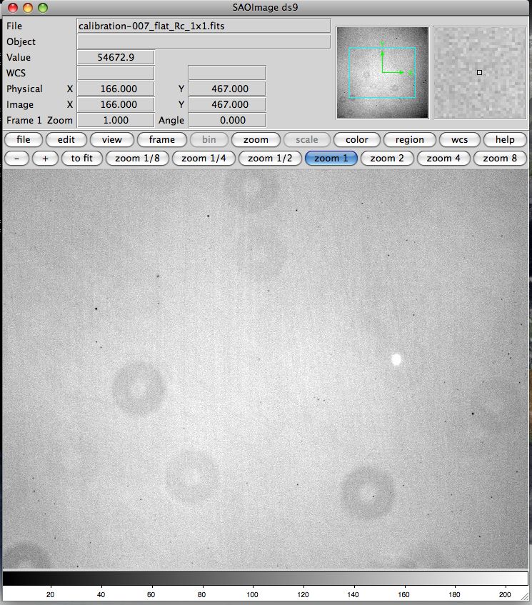
A flat field image taken in the Cousins R filter. Notice the “dust donuts” caused by diffraction of
light around dust particles in the optical path. Other patterns are apparent as well, and these will be in all science images until
they are corrected with a flat field. Click on image for a larger version
|
|
| Bias Images |
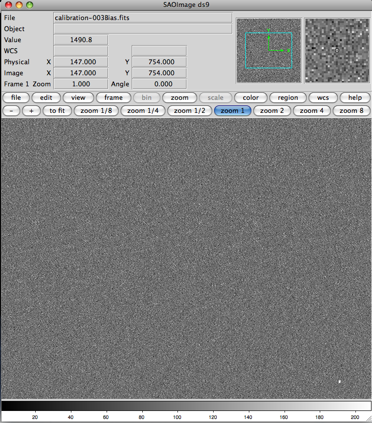
A bias image (sometimes also called a “zero”). Biases are quite smooth, as indicated by the
image. Click on image for a larger version
|
Bias images are used to subtract the bias level for the CCD. The bias level is a nearly constant count level for the chip, often
around 1600 counts. Biases are much easier to make than flats. They are obtained simply by recording an image without opening the
shutter and with a zero second data acquisition time. Basically, they are zero-second dark images (see below). You should take many,
many biases. They should be given names like bias_001.fits, bias_002.fits,
bias_003.fits, etc. Take an odd number of bias images (see the Observing Strategies page for an explanation of why). Usually you can make
bias images by setting the image type in your CCD control software to bias and then telling the controller how
many images to take. Be sure the binning is set to the proper value to match your science images. |
|
| Dark Images |
Dark images are just what they sound like… images taken while keeping the CCD in the dark. This is accomplished by accumulating
data while the camera shutter is kept closed. In most CCD cameras, counts will accumulate even when no light hits the detector. These
counts come from random thermal motions of the atoms in the crystal of the detector. By cooling the chip with liquid nitrogen these
motions can be diminished to the point that the thermal motions are so small that the dark counts become negligible. However, such
cameras require hardware that most amateur telescopes lack, and for this reason we assume most GTN members will make dark images.
In your CCD control software set the image type to dark. You will also have to set the exposure times for your darks. If you
will be making 60 second science exposures, then you want to make darks with at least 60 seconds worth of dark count accumulation. If
you will make 120 second exposures, then your darks should be at least that long. If you want to use 120 second darks with 60 second
science exposures you can scale the dark counts down, though we caution that there is debate about whether this is a good thing to
do. However, you cannot scale 60 second darks up for 120 second exposures. Many people simply make sure that they have dark exposures
that match the exposure time of any science images they will be making. Feel free to use either strategy. If you really want to see if
there is a difference, try reducing your images both ways and check the results. |
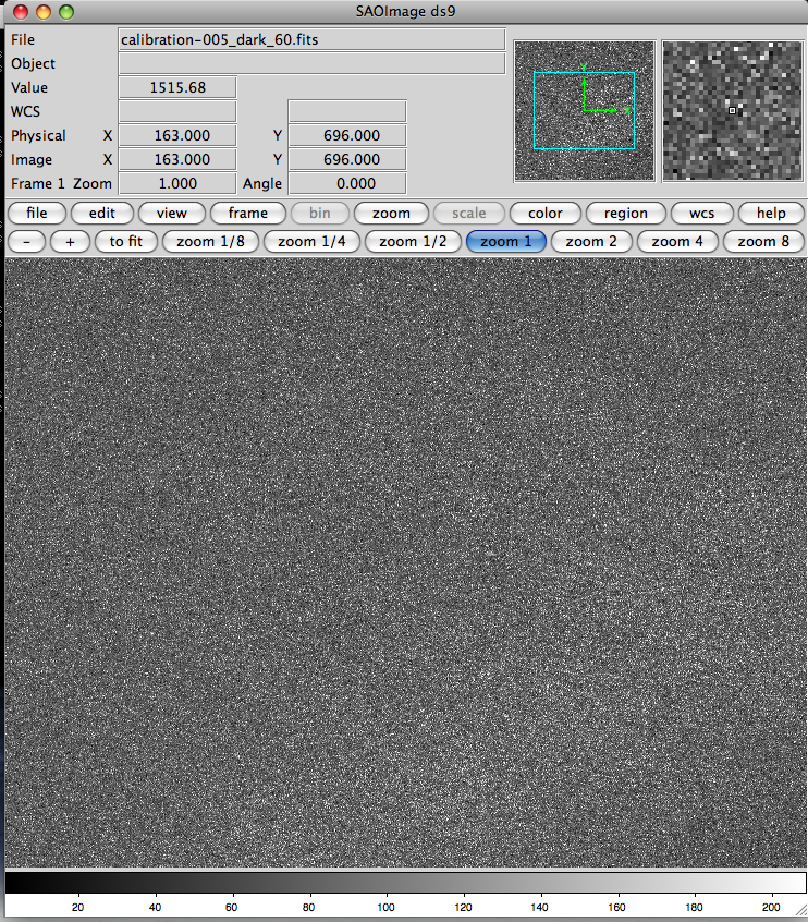
A dark field image, 60 second exposure. The level in a dark image will typically only be slightly higher than a
bias. Click on image for a larger version.
|
Just as for biases and flats, you want to get as many dark images as you can (at various exposure times if you wish). You can then
combine the darks of a given length into a single master dark for that exposure time. Darks can be made in the afternoon before your
observing run, or in the morning following it, so it is not difficult to get lots and lots of them. Like bias images, darks can be
made in great abundance, so you should get as many as you can. Take an odd number, just as you would for other images, so that you can
median combine them into your master darks. Be sure to set the binning so it will match your other images. |
| Automating Calibrations |
Taking calibration images is quite tedious and repetitive. As such, it is a perfect task to give to a computer. Most CCD control software
has some capability to take images automatically. Taking calibration images, especially if you will be making dome flats, is ideally suited
to automation.
When making calibration images you should use the same strategies for naming that
you use for science images. Your CCD control software will generally allow you to choose meaningful base names for your images such
that you can easily tell what an image contains just by looking at it. Below is one possible naming scheme.
	calibration_flat_V_1x1_001.fits
	calibration_flat_V_1x1_002.fits
	...
	...
	calibration_flat_B_1x1_001.fits
	calibration_flat_B_1x1_002.fits
	...
	...
	calibration_bias_1x1_001.fits
	calibration_bias_1x1_002.fits
	...
	...
	calibration_dark_60_1x1_001.fits
	calibration_dark_60_1x1_002.fits
	...
	...
	calibration_dark_120_1x1_001.fits
	calibration_dark_120_1x1_002.fits
These names allow you to instantly know that these are all binned 1×1, and that the first two are flat fields taken in the V filter,
while the second two are flats taken in the B filter. Similarly, we can look at the other files and know that they are biases, taken
with 1×1 binning, and darks, also binned 1×1. It is not important to know the exposure times for biases or flats, so that information is
not used in the names for those images. However, it is important to know the exposure time for dark images, so we have included
it. Notice also that we have left off filter information for the biases and darks; filter information is extraneous for images taken
without any light hitting the detector. Each of the files ends with a number. Usually control software will append a number sequentially
to the base name you choose… It has to do something to distinguish the different files, and numbers are easy and convenient.
The examples given here are one way to keep your images organized for a night. Since you will likely be getting hundreds of
calibration images, and perhaps a comparable number of science images, it is important to do everything you can to keep them all
straight. There are many systems you can use to keep your images organized. Here we just give one example. Use whatever works for
you. Also, be sure to check your calibration images to see that there was not a problem with them… If they are taken automatically
you must check them afterward carefully to make sure they are good.
|
| Summary |
- Be sure to set the binning for all calibration images to the same value you will use with your science images.
- Set the proper image type, flat, bias, or dark when you make each image.
- Get a flat field in each filter you will be using for your science images.
- Try to get as close as possible to saturating your flat fields, without actually saturating any of the pixels. If
the typical value in a pixel (the mode, say) is several thousand counts below saturation that is pretty much ideal.
- Take dark images that are at least as long as your longest science exposure. You might want to take several sets of darks with
exposure times that match each exposure used in your science images.
- Take an odd number of images for each different kind of calibration image so that you can median combine them into a master
calibration image for each type.
- Use meaningful names for your calibration images so that you can easily keep track of them.
|
