
Exoplanets detected by observing dips in the brightness of stars
Credit: NASA Ames Research Center
The brighter planets in our Solar System have been known since ancient times: Venus, Mars, Jupiter and Saturn among them. In the early 1600s, Galileo Galilei used a telescope for the first time to study these planets, and discovered the larger moons orbiting Jupiter, as well as evidence for Saturn’s rings. Studying planets outside our Solar System began in 1995 when Swiss astronomers Didier Queloz and Michel Mayer reported the discovery of the first exoplanet. This discovery was made with a conventional ground-based telescope (at the Haute-Provence Observatory in southern France), but since that time NASA satellites have discovered the vast majority of the exoplanets.
Although NASA’s Kepler exoplanet discovery mission has recently concluded, NASA’s Transiting Exoplanet Survey Satellite (TESS) is still operational. Both Kepler and TESS look for repetitive small changes in the light from stars caused by planets transiting across the stellar disk. To date, over 4000 exoplanets have been discovered. By studying large numbers of planets in other stellar systems, we hope to someday find signs of life in the universe. Click the “Build a Light Curve” link on the top left to continue to the JS9 Activity.
The goal of this procedure is to obtain the relative brightness of a target star with respect to two (or possibly more) comparison stars. Below are two windows: the window on the left shows an image of the target star and two comparison stars. You will use the window on the right to use JS9 to perform the image analysis. First, you will select a region that includes the target star, and measure the brightness in that region. Then you will select each of the two comparison stars and measure their brightnesses. The comparison stars were chosen because they are known to have a constant brightness. By comparing the brightness measurement of the target to the average brightness of the two comparison stars, you will be able to tell if the target star has changed in brightness.
However, there is a limitation with this data analysis approach. – it cannot measure the true brightness of the target, only the relative brightness. Relative brightness is a number which can be close to 0.0 (zero, target is very faint), near 1.0 (one, target is near the average brightness of the comparison stars), or greater than 1.0 (target is brighter than the average brightness of the comparison stars). Measuring relative brightness for a series of images creates a plot called a light curve. Follow these steps to use JS9 to create a light curve for the star as the exoplanet partially obscures its view.
1. Press the T1 (Time 1) Button to load the first image
2. Press the LOG button to make it easier to see the stars. If you click and drag the mouse across the JS9 window you will be able to adjust the contrast of the image.
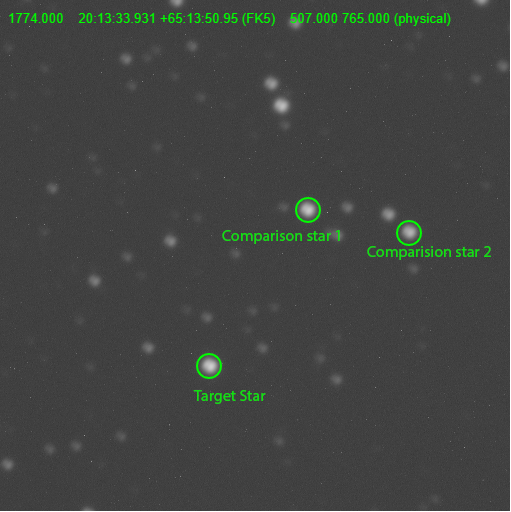
3. On the finder chart below, your target star is in the small green circle closest to the bottom of the chart compared to the other circles.
4. Open the Magnifier Box by pressing the Magnifier Button.
5. Move the Magnifier Box so it doesn’t block buttons or boxes.
6. Press the Add Region Button to load in a circle that you will use to measure the brightness of the target star as well as the brightness of the different comparison stars. Once you have clicked on the circle, use the arrow keys on the keyboard to move the circle more precisely. If you end up with more than one circle click your extra circle and press the delete key on your keyboard.
7. Drag the circle to your target star and click the Target Button.
8. Drag the circle to comparison star 1, as shown circled and labeled on the finder chart and click the Comp 1 Button.
9. Drag the circle to comparison star 2, as shown circled and labeled on the finder chart and click the Comp 2 Button.
10. Click the Plot Button to plot the relative brightness, which is the regional pixel count of the target star divided by the average of the regional pixel counts of the comparison stars. The plot is drawn under the finder chart and JS9 window.
11. Repeat these steps for each of the available images taken at different times, (T1-T5).
Finder Chart
Region Pixel Counts:
If you think you understand the data analysis steps, you can have the rest of the points drawn on the plot by clicking the Draw Complete Chart button below. If you want more practice, close this box and continue selecting data. You can always click on Complete Chart button above, if you change your mind. If you do not wish to have the chart auto complete click anywhere outside of the textbox to close this prompt.