
The Lives of Stars
|
“… we would never know how to study by any means their chemical composition, or their
mineralogical structure…”
–Auguste Comte, 1798-1857 |
The partial quote above, by the 19th century French philosopher and theologian, Auguste Comte, provides an example of the perils of predicting the future. He went on to speculate further that, just like their composition, we could never know the temperatures of the objects to which he referred.
The objects were the stars, and within only a few decades of these pronouncements, scientists
had increased their knowledge of physics to the point that questions about the stars, their
compositions, temperatures and many other properties, could be addressed meaningfully. A
century after that, the chemical composition of stars – and much else about them – was
substantially understood.
In this brief article we will come to know how a knowledge of the stars and their makeup was
completed. We will see how it is the stars that are responsible for the creation of nearly all the
chemical elements, on Earth and beyond, and how the production of the elements is
inseparably linked to the lifecycles of the stars.
Introduction
If you live in a place far from cities or towns, where the night sky is moderately dark, you will have noticed the tiny points of light dotting the heavens – the stars. If the moon is not up, you can see several hundred to several thousand stars at any given time. However, in the city, the brightness of the environment, caused by streetlights, headlights of cars, billboards and other artificial lights, drops the number of visible stars to only a few dozen. In many locations only a handful, or even fewer, can be seen. Maps like that in Figure 1, taken by Earth-orbiting satellites, illustrate the effect electric lights have on the night sky. In the areas where towns are packed tightly, the skyglow at night blocks a view of the stars. In the United States, only in a few areas in the West do the skies retain their pristine nighttime darkness.
Despite the relatively recent increases in sky brightness, for preceding millennia people looked up and wondered at the nature of the stars. They were able to record the patterns they saw, and they understood that the patterns varied gradually over the year. Some stars are visible in winter, others in summer. And when travel between locations above the equator and below became common, people also realized that an entirely different set of stars is visible from locations in the far south as compared to the far north.
All of this was discernible by observing the sky with the naked eye, unaided by any technology. However, once devices like telescopes, cameras and especially spectroscopes became available, a wholly unimagined understanding of stars became available.
Planck Spectra
The spectrum emitted by stars is essentially a Planck spectrum. This is the spectrum emitted by light that is in thermal equilibrium with the matter around it. The spectrum is quite distinct from other kinds of spectra, and it can be described by a single parameter: the temperature of the emitter. The Planck spectrum plays a central role in our understanding of the origin of the universe, which is discussed in the History and Origin of the Universe‘s chapter on The Primordial Background Radiation.
Planck spectra for several emitting objects at different temperatures (3000K, 4000K and 5000K) are shown in Figure 4. The spectra are shown as a graph, with brightness on the vertical axis and wavelength on the horizontal one. If we displayed these photographically, as was done with the stellar spectra in the previous section, we would see only a featureless rainbow. There would be no dark lines. Also, the distribution of energy with wavelength would not be clear. Only plotting a spectrum as a graph allows us to see this distribution.
There are two features to note with Planck spectra. First, as the temperature of the emitter increases, its spectrum grows higher at all wavelengths, meaning it is radiating more energy per unit area per unit time for all wavelengths. Second, the peak emission, the highest part of each curve, shifts to shorter wavelengths as the temperature goes up.
If we were to plot the spectrum emitted from the surface of a star on a graph, similar to these plots, it would look very much like these Planck curves. One notable difference would be the presence of the dark lines in the stellar spectra. Figure 5. provides examples of exactly these kinds of plots for stars with spectral types ranging from O to G. K and M type stars are not shown.
That the different stars in the figure have different Planck curves is not apparent when displaying the spectra photographically. However, the brightness vs. wavelength format makes this immediately apparent. The theoretical explanation of Planck curves was not understood until 1900, around the same time that Annie Cannon was completing the system of stellar classification. So the relationship of temperature to spectral class was not recognized at first. However, the changing pattern of the dark lines seen in the previous figure is directly related to the increase in temperature of the stars from bottom to top. The importance of this fact was not appreciated until the mid 1920s, and when it finally became known, it revolutionized the way astronomers understood the material content of the cosmos.
Line Spectra: Absorption and Emission by Atoms
While astronomers were devising systems of stellar classification, physicists were busy
studying the emission of light by hot gasses in their laboratories. Gasses heated to very high
temperatures glow, as we know from experiences with emission tube lighting. We often call
these types of lights “neon signs,” though that is a somewhat misleading label.
Hot gasses do not glow in the same way that a Planck emitter does. They do not produce a smooth rainbow of emission. Instead, when light from a hot gas is passed through a spectroscope, we see a collection of discrete bright lines. Figure 6 provides examples of this emission spectra for various elements.
Other gasses show similar patterns of lines. Spectra of this sort are called emission spectra,
because the hot gas is emitting light. Several general properties and trends are apparent in
emission spectra of different types of gasses.
- Each kind of gas has a unique spectrum. Hydrogen is different from helium, which is
different from oxygen, which is different from neon, and so on.
- More complicated atoms (atoms with more electrons) tend to show more complex
spectra. So as one progresses up the periodic table from hydrogen, which has a
single electron, to helium, with two electrons, to heavier atoms like nitrogen,
oxygen, neon, sodium and so forth, the emission spectra tend to contain more lines.
The examples above illustrate this trend dramatically, as sodium has 11 electrons, as
compared to hydrogen’s single electron.
- A given type of atom always shows the same pattern of lines, so the pattern of lines
seen in a gas provides enough information to uniquely identify the kind of gas
emitting the light.
Physicists did not only look at the spectra emitted by hot glowing gasses. They also passed white light through gasses so that they could observe the effect the gas would have on the
light as it passed through. What they found was interesting, and not at all surprising in retrospect. Passing white light through a gas produced what was called an absorption spectrum.
Figure 6 also shows the pattern seen after passing white light through various elemental gases and then through a spectroscope. Now we see the rainbow, characteristic of full-spectrum white light, but with gaps. If you compare this spectrum to the emission spectrum for the gases shown, you will see that the pattern of dark lines in the absorption spectrum exactly corresponds to the pattern of bright lines in the emission spectrum. Other gasses show the same effect: if you pass white light through a gas you will see a pattern of dark lines that exactly matches the bright line pattern seen in emission spectra.
The absorption spectra seen in laboratories is the same as we see in the spectra emitted by
stars. Apparently, those spectra are produced by passing white light through layers of
intervening gas. Hot layers deeper in a star’s atmosphere emit the rainbow of white light, and
cooler, thinner layers above absorb some of the light to form the absorption spectrum. So what
is happening in that gas?
As we know now, but scientists in the 19th century did not know, these bright and dark lines correspond to electrons in atoms changing their energy states. In the emission spectra, collisions between particles in the hot gas promote electrons from their lowest energy state (called the ground state, and where they are found if left alone) into higher energy states, called excited states. The electrons do not spend very much time in the excited states. They typically transition back to the ground state after roughly `10^8s`. When electrons make this transition, light is emitted, and the energy of the light (related to its wavelength) is exactly the energy difference between the two states.
Several of the energy levels in hydrogen are shown schematically in Figure 7. These correspond to the four brightest lines seen in the visible part of the spectrum. There is one energy level below those shown. It is the ground state of the atom. However, we have omitted it because it does not participate in the visible spectrum; all the transitions to the ground state are in the ultraviolet.
To make sense of this diagram, note that electrons are excited from one of the states shown into a higher state by a collision, assuming there is an electron in the state to begin with. These transitions are suggested by the white arrows on the left. Electrons from the ground state can also be moved into one of these states. The electron then de-excites, emitting a photon as it does so. These de-excitations are represented schematically by the colored arrows. On the right, the quantum number, n, is shown for each state (the ground state, not shown, has n=1), and the wavelength of light emitted is also shown in the color corresponding to the arrow showing that transition. The energy of the light (in electron-volts) is shown for each as well. All the visible transitions terminate on the n=2 level, which is the first excited state of the atom.
These energy levels and their spacings are unique to hydrogen. We could have made a similar diagram for any other atom. It would have been qualitatively the same, but the pattern of
available energies would have been different for each of them. As a result, a unique pattern of emission lines would be produced by different kinds of atoms. That is why the emission and absorption spectra are different for each type of atom.
None of this physics was understood until the 1920s, but scientists were aware of the peculiar aspects of the spectra in atoms long before that, in the middle of the 19th century. So it was not long before they noticed that the patterns seen in the spectra of gasses in labs was also seen in stars. Except star spectra are mixtures of lines from different kinds of atoms, they are not the spectrum of an isolated atomic species. In the Sun, for example, there are prominent lines of calcium, sodium, magnesium and other atoms. The vast majority of the lines in the solar spectrum turned out to be from iron. These same lines are seen in the spectra of other stars, too.
See the Additional Resources tab on the left.
Stellar Spectra and Classifications
A spectroscope is a device that splits light into its constituent colors. It had been known for
ages that this was possible; a rainbow is the most obvious example, and they are seen by just
about everyone. However, only when physicists began to study light carefully did an
understanding of this property of light begin to emerge.
Through the work of scientists in the 17th and 18th centuries, light was understood to have a
wave-like nature. The different colors of the rainbow are made by light with different
wavelengths. The longest wavelengths appear red. The shortest wavelengths are blue/violet.
Wavelengths in between are orange, yellow and green. This spectrum of light is what allowed
the study of the stars, and almost everything else far from Earth, to be undertaken.
Figure 2 shows a high resolution spectrum of the Sun; sunlight has been passed through a
spectroscope and recorded by a camera. The rainbow color spread is clearly visible, but also notable are many dark
vertical lines dotting the spectrum. We cannot see these lines when we look at a rainbow
because they are smeared out too much. However, under more controlled conditions it is
possible to create an “artificial rainbow,” in a sense, in a laboratory. Then the lines become
quite noticeable.
By the middle of the 19th century astronomers had begun to connect spectroscopes to their telescopes. They found that, just like the Sun, the stars showed patterns of dark lines. In some stars the patterns were similar to the one seen in the Sun. Other stars showed markedly different patterns. In order to understand the confusing array of lines, systems of classification were developed based upon the lines.
The most extensive spectral classification of stars was done at the Harvard College
Observatory. As we discussed briefly in the History and Origin of the Universe section of this site, the observatory
did much of the early work that underlies our current understanding of the universe. This was
nowhere more true than in unraveling the mysteries of the nature of stars.
The image below shows the classification of stars that was finally settled upon. It was the
culmination of years of work by several Harvard astronomers, including Williamina Fleming,
Antonia Maury, and especially Annie J. Cannon. The Harvard classification system had
antecedents elsewhere, but it was the extensive and systematic work done at Harvard that
finally provided true insights into the workings of stars. The classification system settled upon
by Cannon has needed only minor revisions since she developed it around 1900.
To understand Cannon’s classification system for stars, look at the lefthand side of figure below. It has labels running from O6.5 at the very top to M5 at the bottom. In between are
various labels running through the letters B, A, F, G and K, each with a number appended to its
right side. These are the star classifications. They run through a sequence, OBAFGKM, with a
numeral from 0 to 9 (with decimal fractions of tenths) providing finer divisions. The three bands
at the bottom are peculiar stars; they do not fall neatly into the standard classification system.
Now look carefully at the image. You see a series of horizontal rainbow bands. These are the spectra of individual stars of the type indicated. The catalog designation for each example star is also given, on the far right side. Each star’s spectrum has the characteristic vertical dark lines, just as in the Sun. Keep in mind that different colors correspond to a different wavelength of light. As you sweep your eyes from the top of these bands toward the bottom (ignoring the last three) you will notice that the lines change. Some lines get stronger at first, and then weaken and disappear. Other lines appear at wavelengths where originally there were none.
Near the top, in classes A and B, there are strong lines in the blue part of the spectrum. These
lines are less pronounced in the O stars, and also in types F, G and below. They never quite
disappear though. Similarly, there is a very strong line in the yellow/orange part of the spectrum
for M and K stars, but that line becomes much weaker (though still present) in the stars above.
What does all this mean? It helps to have one additional piece of information that is not
obvious looking at this image.
Stellar Composition
When Annie Cannon and her colleagues were creating their stellar classification schemes, they
had no idea how the lines were produced. They saw systematic patterns in the lines and classified the stars according to those patterns. Clearly, stars must contain atoms of the type
revealed by the spectra, but no one knew in detail how the lines were produced. It was natural
to assume that, if a larger number of lines was seen from a given type of atom, or if lines
related to a certain atomic species appeared stronger, then a star must contain more of that
kind of atom. Taking the concept further, if a star did not contain the lines of a particular type of
atom, then it was only natural to assume that the star did not contain that type of atom.
While this reasoning was all purely natural, and it is what most astronomers of the day thought,
it was also completely wrong.
By the early 1920s, the understanding of atoms had progressed to the point that scientists
could apply quantitative methods to the study of stellar spectra. A young British scientist at the
Harvard Observatory did exactly that. Her name was Cecelia Payne, and she had come to
study at Harvard after completing her physics undergraduate degree in Cambridge, England.
Payne applied the relatively new insights into the quantum statistics of atoms to understand
why the lines in star’s spectra had the strengths they did. What she found shocked her, and
everyone else.
Cecelia Payne found that, upon careful analysis, the number and strengths of the lines in stellar
spectra had essentially nothing whatsoever to do with a star’s composition. It was entirely
related to the surface temperature of the star, the temperature of its corresponding Planck
curve. Her work showed that all stars have essentially the same composition, with only minor
variations. They are about 90% hydrogen atoms (by number) and 10% helium atoms. That left
approximately 0% for everything else.
Why, then, are most of the lines that we see in the spectra of stars created by absorption from
many other kinds of atoms, but almost none of them are from hydrogen or helium? To be sure,
hydrogen does form extremely prominent absorption lines in some stars, particularly A stars. In
those stars it is essentially the only absorption seen. But hydrogen is almost (or completely)
absent in many other stellar spectra, where heavier elements are seen in abundance. What is
the cause of this puzzling phenomenon?
The answer, in a word, is temperature. As the temperature increases, the excitation levels of the
atoms in a star’s atmosphere go up accordingly. Some of the electrons are even completely
separated form their atoms in a process called ionization. Ionization occurs in atoms when the
energy in the collisions in the gas, or in the radiation, is comparable to the energy binding
electrons to a nucleus.
Have a look again at the schematic energy level diagram for hydrogen. Notice how the higher excitation levels tend to bunch together near the top of the figure. There are large steps from the ground state (n=1, not shown) to the first excited state with n=2. The step from the second to third (n=3) state is smaller, and the next one, from n=3 to n=4 is smaller still. This pattern continues for all higher energies.
There is a simple mathematical relationship that expresses the energy difference between states, and it is shown below. It is a form of the Rydberg formula.
The equation gives the energy difference (in electron-volts) between two states, labeled `n_i` and `n_f`, for initial and final states for a particular transition. It also, therefore, gives the energy of light emitted/absorbed when the electron moves between these energy levels. The Rydberg formula
only describes hydrogen quantitatively, but it gives a correct qualitative picture for other kinds
of atoms, too.
The only condition on the quantum number n is that it be a positive integer. So it can run from 1
upward without bound. Notice, though, that as `n_i` or `n_f` becomes larger, the corresponding factor tends to zero. So if we imagine starting at the ground state of the atom, `n_i= 1`, moving to
the state with `n -> oo` corresponds to an energy of 13.6 eV. That is the amount of energy we
have to provide the electron to promote it to the highest, barely bound state. Any additional
energy will unbind the electron from the atom.
The energy required to unbind an electron is called the ionization energy of the atom. For
hydrogen it is 13.6 electron-volts. This is higher than the energy of visible light by a factor of
four or five. A similar process can happen for any atom, but the ionization energies tend to be
much lower, in the visible wavelengths. Of course, the visible wavelengths are also the energies
of much of the light emitted by stars, even the coolest stars.
In order to understand stellar spectra and the results of Cecelia Payne, imagine what happens
to hydrogen atoms as we move from the coolest stars to the hottest stars.
In the coolest stars, the M stars, the temperatures are around 3000K. These stars are so cool
that their Planck curves peak in the infrared (IR) part of the spectrum, not the visible. At these
temperatures all the hydrogen at the stars’ surface is neutral and substantially in the n=1 state,
the ground state. There is simply not enough energy available to excite most hydrogen atoms
to higher states and keep them there.
How do we know this is the case? We can use the Rydberg formula to compute the energy needed to promote electrons from n=1 to n=2 as an illustration.
The energy is well into the the ultraviolet (UV) part of the spectrum. M-type stars produce
almost no UV radiation. Nor do the atoms in a gas at these temperatures tend to be moving
fast enough to promote to this level through collisions. That is what radiation in equilibrium with
matter means; the typical energies for the matter and the photons are the same. As a result, in
M-stars we do not tend to see absorption of hydrogen in the visible part of the spectrum.
Recall that the visible light emission lines result from transitions terminating on n=2, so the
corresponding absorption lines originate there.
As the stellar temperature goes up, collisions become more energetic. Eventually the population of electrons in the n=2 state increases, and these electrons begin to absorb light
before they can decay back down to the ground state. At this point, weak hydrogen absorption lines are seen in visible light. Look for dark vertical lines running through the A star spectra in figure 3. The two strong dark lines on the left are hydrogen absorption lines. You will notice that the dark lines at these energies are not found in the M star spectra. Other dark lines at other energies indicate absorption by other elements.
As the temperature rises through F to A, the hydrogen lines become very strong because we
are adding more and more electrons into the n=2 state via collisions. Then a strange thing happens; they weaken again in the B-stars, and in the O-stars they are almost gone. What has
happened? Ionization.
A-type stars are hot enough, around 10,000K, that they begin to appreciably ionize the
hydrogen in their atmospheres. The atomic collisions in these stars are so energetic that they
can promote electrons from the n=1 state (and all the other states, of course) completely out of
the atoms. B-stars are hotter still, around 20,000K, and O-stars are even hotter, 40,000K or
more. As a result, in these hottest of stars, many of the hydrogen atoms cease to exist. They
are converted to free protons and free electrons. As a result, the hydrogen absorption gets
weaker and weaker and finally goes away entirely.
Analogous processes occur for all the atoms in the atmospheres of stars. For the lowest
temperature stars, of types M through G, many atoms remain neutral and in their ground states
for the most part. But as temperatures get higher, the atomic excitation increases, and various
lines appear and disappear. By the time the A-stars are reached, nearly all the atoms have lost
at least one electron, and sometimes two. This is because the outer electrons of most atoms
are not as strongly bound as the electron in hydrogen is. So only hydrogen is left to absorb
light in the hottest stars, and only the absorption lines of hydrogen are seen as a result.
The line formation process depends sensitively on both the relative abundance of different
atoms and on the temperature of the gas. It was the critical temperature dependence that
Cecelia Payne discovered. With it, she overturned the conventional wisdom about the
composition of matter in the universe.
Payne published her results in 1925, but her contribution was not immediately apparent or
appreciated by her contemporaries. The new quantum statistics was not understood by
everyone, and the eminent astronomer Henry Norris Russell even dissuaded Payne from
emphasizing her findings. Unfortunately, the fact that she was a woman in a very maledominated
profession did not help, either. Eventually the veracity of what she had found was
recognized.
For her monumental achievement, the then-director of the Harvard Observatory, Harlow
Shapley, wanted to award Payne a PhD. It would be the first time a doctorate would be
awarded to one of the women working on astronomical projects at Harvard Observatory,
though certainly Payne’s work was not the first to be worthy of the degree.
Up to that time, PhDs for astronomical work at Harvard were awarded by the physics
department, to which the observatory was attached. However, the Chair of the physics
department refused to award a doctorate to a woman, regardless of the research contributions
she had made. So Shapley appealed to the president of Harvard to make the observatory its
own academic department. He could then award a well-deserved doctorate to Cecelia Payne.
Thus was born the Harvard Astronomy Department, and thus was the first of its doctoral
degrees awarded. Cecelia Payne would become one of Harvard’s first astronomy faculty, and
she would eventually become its chair. She retained her position until her death in 1979,
training many students during her tenure.
While Cecelia Payne (later to be Cecelia Payne-Gaposhkin) discovered the composition of the
stars, neither she nor anyone at that time understood the origin of all the various atoms within
them. That understanding had to wait another decade, and for the efforts of a young German
physicist who, while on a convalescent stay at a spa in the south of his country, was puzzling
over the details of a different mystery entirely: the manner by which stars, and particularly the
Sun, power themselves.
It turned out that the questions of composition and energy generation are intricately entwined, but no one knew it then.
See the Additional Resources tab on the left.
The Formation of the Chemical Elements
Aside from a few of the lightest elements, hydrogen, helium, lithium and sprinkling of others,
the story of the origin of the chemical elements is the story of the formation and evolution of
the stars. Because it involved all four of the known interactions, gravity, electromagnetism and
the strong and weak nuclear interactions, the story could not be written until relatively recently.
After all, until the early years of the 20th century, nobody even knew of the existence of the two
nuclear interactions, or even that the nucleus existed!
We will describe the early attempts to understand the power output of the Sun in order to set
the proper context. After, we will outline how the eventual understanding of the true means of
solar (and stellar) energy production came about.
Powering the Sun
By the middle years of the 19th century, the power output of the Sun had been measured. It is
not a difficult task if one knows how far away the Sun is from Earth. By measuring the solar flux
at Earth’s surface, and then using some geometry, the solar power output can be computed.
The geometry is called the inverse-square law. It is described on the page about the Early
Universe if you want to know how it works. We will illustrate the computation below.
The amount of energy received at the top of Earth’s atmosphere, called the solar constant, is
1388 watts per square meter. This is the current value, measured by satellites orbiting above
Earth and free from atmospheric effects. Historically, the value was measured at Earth’s
surface. The atmosphere absorbs and reflects some of the energy radiated by the Sun, so a
measurement done at the surface will not count this missing energy and will be somewhat
lower, by around ten or fifteen percent, than the true value.
We will assume that the energy emitted by the Sun is essentially constant in all directions, a characteristic called isotropy. We can further imagine the Sun is surrounded by a huge spherical surface of radius `r`, and that the two are concentric. All the energy emitted from the surface of the Sun must pass through this imaginary surface. If the energy radiated by the Sun is isotropic, then the flux, `F`, is constant everywhere on any spherical surface surrounding it, and we can describe the flux at any point on the surface by the relation below.
We use `Lodot` to represent the total energy output of the Sun. The denominator on the right hand side is the area of the sphere surrounding the Sun. If the luminosity is measured in watts (joules per second) then the flux could be in watts per square meter (`Wm^-2`).
Setting the flux equal to the solar constant, and using the size of Earth’s orbit for `r` (`1.49 x 10^11 m`), we can compute the luminosity of the Sun.
Clearly, this is a lot of power. It is 100 trillion trillion joules per second, enough to light a trillion trillion 100 watt lightbulbs. In the 19th century, there were only two sources known that could be providing the energy. One was combustion, the burning of material by combining it with oxygen. The other was gravitational contraction. It is not difficult to show that combustion cannot account for the enormous energy output of the Sun, but we will not do that calculation here. Instead, we will look at how the energy production from gravitational contraction, which far exceeds that of combustion, still completely fails as an explanation for the Sun’s luminosity.
The estimate below of the Sun’s gravitational lifetime recapitulates one done toward the end of the 19th century by William Thomson (later Lord Kelvin, for whom the kelvin temperature scale is named) in England. At the time, the mass of the Sun was known to be approximately its current value, `2 x 10^30kg`. The Sun’s radius, 700,000km, was also known reasonably well. Given these two pieces of information, the total gravitational energy available to the Sun is given by the expression below. We will plug in the values for the mass and radius and thus find the amount of energy the Sun has in the form of gravitational energy. The symbol `G` is called the gravitational constant. It has a value of `6.67 x 10^-11 Nm^2kg^-2` and merely keeps track of the system of units we are using.
This is lot of energy, too. To find out how long it could power the Sun at its current output we divide the total energy available by the energy emission rate.
Using the fact that one year is about 30 million seconds, we find that the gravitational timescale for the Sun is around 30 million years. This is how long the Sun could shine if all its
luminosity was produced by gravitational contraction.
This timescale is far too short. Already in the late 19th century, geologists had strong evidence that Earth was at least several hundred million years old by measuring the ages of rocks. Clearly, Earth must be as old as its oldest rocks. Since then, even older rocks have been found. We have now measured the ages of rocks on Earth and some are as old as four billion years. It seems unlikely that Earth is older than the Sun, so gravity cannot account for the energy production of the Sun. It fails to do so by many orders of magnitude.
That is where the problem stayed until the 1930s, by which point new physics was known. As with the mystery of stellar spectra and chemical abundances, applying new physics to an old problem yielded positive results fairly quickly.
Hydrogen Burning
While scientists had made progress understanding gravity and electromagnetism by the turn of the 19th century, the nature of the atom was not at all understood at that time. They knew that matter was composed of independent substances, the chemical elements, that combined to form various materials, the chemical compounds. And they knew that these various elemental substances seemed to be made of indivisible units they called atoms. However, the nature of those elemental, and possibly indivisible, bits of substance was a topic of debate.
The first revelation of the true nature of atoms came in 1911, when scattering experiments by
the Canadian physicist Ernest Rutherford demonstrated that essentially all of an atom’s mass is
concentrated in a tiny, positively charged region at its center, now called the nucleus. The
negative electrons occupy a vastly larger area that constitutes something that could be
considered the “size” of the atom, but that contains essentially none of its mass. So atoms are
not indivisible, they are composed of smaller bits.
Further advancements in understanding of the atomic nucleus led to the discovery of protons
by Rutherford in 1917, and of neutrons by James Chadwick in 1932. These discoveries showed
that the nucleus is itself composed of two kinds of subatomic particles. The proton has a
positive charge, and the neutron has no electric charge at all. The neutrality of the neutron
makes it ideal for probing the nature of the atomic nucleus, because its lack of electric charge
allows it to penetrate to the nucleus without having to overcome the strong interactions
between electrically charged particles.
Neutrons were subsequently put to use by three German scientists, Otto Hahn, Fritz
Strassmann and Lise Meitner. They used neutrons to bombard uranium nuclei, thinking to
create uranium nuclei of heavier mass (called isotopes) through absorption of the neutrons.
Instead, they found that they created barium, a much lighter nucleus, by splitting the uranium
atom into two parts. Their discovery of nuclear fission in 1938 demonstrated that it is possible
to change one type of atom into another type with the release of energy. Induced nuclear
transmutation had been accomplished previously, but not with the net release of energy.
It turns out that neutrons are not stable outside of an atomic nucleus. They decay to a proton (`p`), electron (`e^-`) and an antineutrino (`overline v_e`) – the bar over the neutrino symbol differentiates between a neutrino and an antineutrino. The reaction is shown below.
Neutron decay is the fundamental type of beta decay. It is given this name because the
electrons emitted by the process were historically referred to as beta rays; at the time it was
not understood that they were actually the already-known electrons. The reaction was originally
observed in certain radioactive nuclei, in which it will have a timescale that is distinct for each
isotope. For free neutrons (those outside a nucleus), there is a 50% chance of undergoing beta
decay in about 11 minutes. So we say the reaction has a half-life of 11 minutes.
Nuclear fission is one way to extract nuclear energy. This is done by breaking (certain) atoms
apart. Some scientists wondered if there is also a way of extracting energy by fusing nuclei –
putting them together. Fortunately, there is such a way. Under suitable conditions, the opposite
of the neutron decay just described can occur, and a proton can convert to a neutron. This is
key to understanding how to build up heavy nuclei from lighter ones, and to understanding
how to power the Sun by these sorts of fusion reactions.
The most obvious mechanism for nuclear energy production in the Sun would be the conversion of hydrogen, which as we have seen, accounts for 90% of the Sun’s atoms, into helium. A simple calculation shows that this can work, at least in principle. To see why, we will compare the mass of two protons and two neutrons to the mass of a helium nucleus (an alpha particle), which contains two protons and two neutrons.
Note that the mass of the alpha particle is smaller than the combined mass of its constituent parts. How is this possible? When combining the two protons and neutrons into an alpha particle, some of their mass is converted into binding energy. This amount of energy, described by Einstein’s famous `E = mc^2`, is released when the alpha particle is formed. It is also the amount of energy that must be provided to break the alpha particle up into its constituents again.
So, is this a large amount of mass, or a small amount? If we compare the mass lost to the amount of mass at the beginning we see that quite a large amount of mass is lost. We find the fraction of mass lost using the expression below.
Approximately 0.7% of the mass of the initial particles is converted into energy when protons and neutrons are combined into an alpha particle. That is almost 1%!!! But again, is this a lot of energy, and is it enough to power the Sun? To find the answer, we must use Einstein’s equation to convert mass to energy.
This doesn’t look like a lot of energy, but then, it comes from converting only a fraction of a proton mass into energy. Protons are not very big. On the other hand, the Sun has a lot of protons in it. The important question is how long can the Sun shine if it converts this fraction of every proton into energy, or put another way, if it converts about 0.7% of its mass into energy. We can answer that question by doing the same computation we did before when we found the gravitational timescale of the sun. This time we will use the nuclear energy available to find the nuclear timescale.
The nuclear timescale for the Sun is considerably longer than the gravitational timescale. We
can convert it to years by dividing by `3.155 x 10^7s yr^-1`. We then have a much more
reasonable timescale: 100 billion years. That is easily older than Earth, so it does not run into
the problem that the gravitational energy generation rate did. Even if the Sun only ever converts
10% of its hydrogen to helium, which seems reasonable, we still have 10 billion years. This is
easily enough time to explain the Sun’s (and Earth’s) current age. But beyond that, how can we
be sure this happens?
To make additional progress we have to understand the nuclear reactions by which the Sun converts hydrogen to helium. This was done by the German physicist Hans Bethe (pronounced like beta) in the 1930s. The reaction chain he worked out for the Sun is called the proton-proton chain, and its steps are listed below, though some variations on these are also possible.
Note that in the first step, two protons are combined into a deuteron, a heavy nucleus of
hydrogen with one proton and one neutron. In this step, one of the protons converts into a
neutron, reversing the neutron decay process we saw earlier. Additionally, the antiparticle of an
electron, called a positron, is also created, along with a neutrino – in this case it is a neutrino,
not an anti-neutrino. (From now on we will not necessarily distinguish between neutrinos and
antineutrinos because their differences are not particularly important for our context. We will
simply say neutrino for both.) This process releases energy, which is carried by the positron
and neutrino, plus any kinetic energy of the deuteron.
In the second step, a proton combines with the deuteron to form a light isotope of helium
called helium-three. It contains two protons (that is what makes it helium) but only a single
neutron. This process also releases energy, and that energy is carried away by a gamma ray
(i.e., a photon).
In the last step, two `overset3` `He` nuclei combine to form `overset4` `He` (an `a`-particle), with the release of 2
protons, which can begin the process again. Note that in net, the reaction chain converts four
protons into an α-particle, with a release of energy. The positron annihilates with an electron
(those are everywhere in the Sun) and the two are converted to photons.
The energy released by these reactions is what heats the solar interior and provides the
pressure needed to support the sun against gravitational collapse. The photons very slowly
diffuse outward, where they are eventually emitted at the surface: sunlight! As we have seen,
without this source of energy, the Sun would collapse on a gravitational timescale, only about
30 million years.
But what of the neutrinos? Those do not remain in the Sun. Neutrinos have a minuscule
probability to interact with matter. So minuscule, in fact, that the Sun is essentially transparent
to them. The neutrinos go streaming out in all directions, some of them toward Earth.
Physicists have set up experiments to try to detect them, and for many decades were puzzled
because they found only a third of the expected number. Discussions ensued about the possibility that the Sun’s interior might have (for some unknown reason) stopped its nuclear
reactions, or that our understanding of nuclear physics was simply wrong.
The resolution of the problem turned out to be related to the latter: our understanding of
neutrinos had been incomplete. We know now that, on their way from the Sun to Earth,
neutrinos change from the type created in the Sun (they are called electron neutrinos. That is
why they have the little “e” subscripts) into two other types in a process called neutrino
oscillation. Our solar neutrino experiments are not sensitive to these two other types, hence we
are able to detect only one third of the total neutrinos produced, those that remain electron
neutrinos. As often happens, new physics and new understanding is needed to fully grasp a
new phenomenon.
In stars like the Sun, the p-p chain dominates energy production. For the reactions to occur,
the interior of the stars must be unimaginably hot, in excess of 4 million kelvin. Only then will
the protons be moving fast enough to overcome their electrical repulsion to one another. And
overcome this they must. In order for the nuclear interaction to dominate over the electrical
interaction, the protons must come within `10^15 m` of each other.
In slightly more massive stars, those with masses about 30% greater than the Sun, a different
process begins to take over. It is the dominant hydrogen conversion process in the most
massive kinds of stars. The process is called the CNO cycle, for carbon-nitrogen-oxygen. Don’t
be confused by the name though, the process converts hydrogen to helium, just as the p-p
chain does. However, the reactions are catalyzed by C, N and O. That is why it has been given
its confusing name.
The reactions of the CNO cycle are more complicated than the reactions in the p-p chain. In fact, there are really several different CNO cycles that have slightly different branches and routes. But they all produce a helium nucleus from four protons. The reactions of one of the cycles is shown below as an example.
The reaction chain is shown schematically in Figure 8. The cycle begins with `overset12` `C`. It consumes four protons, and these are eventually spit out at the end as a nucleus `overset4` `He`, along with a `overset12` `C`. The chain is then ready to resume with additional protons as inputs. Only protons are consumed. The other atoms undergo no net change in number. That is why we say that C, N and O catalyze the hydrogen fusion process.
The CNO cycle can only occur at extremely high temperatures because it is necessary to overcome not just the electrical repulsion between two protons, but between a proton and a C, N or O nucleus. The larger positive charges of these nuclei create a greater repulsive force. As a result, CNO cycle fusion does not happen in stars smaller than the Sun. Their core temperatures, in the vicinity of 4 million K up to 15 million K, are simply not hot enough. The CNO cycle requires temperatures above 15 million K to occur. In stars with temperatures higher than 15.7 million K (the core temperature of the Sun, it turns out) CNO dominates over the p-p chain. Both reaction processes have strong temperature dependences, but the CNO temperature dependence is much stronger than the p-p chain dependence. As a result, for the most massive stars the CNO cycle takes over. Keep in mind that both are occurring in massive stars, but CNO is responsible for by far the bulk of the energy output.
This CNO process has an important affect on the relative abundances of carbon, nitrogen and
oxygen in the universe. Each of the steps in the CNO cycle (including the two other branches
that we have not shown) has a unique timescale. Some of them occur very quickly, but others
are comparatively slow. The steps that happen quickly totally consume their input nuclei while
waiting for the slow steps to complete. So some of these nuclei pile up and their abundance
goes up. Others are consumed and so their abundance is low. The important point is that the
timescales for the steps, which are set by nuclear physics, determine relative abundances of
these isotopes of carbon, nitrogen and oxygen. The abundances can be observed in stars and
gas clouds throughout the cosmos. So we have a theoretical prediction (relative abundances of
C, N and O isotopes) of an easily observable quantity, allowing us to test whether or not the theory of energy production matches our observations of the world. In this case they match
very well.
Through this check we have high confidence that the CNO cycle does indeed power the
massive stars in the universe. Hans Bethe and Carl von Weiszäcker were the first people to
work out these chains. They did so independently in the late 1930s, Bethe while convalescing
at a spa in Germany. Thus they were the first persons in history to understand why the stars
shine as they do.
The reaction rate in stars is finely balanced. If the rate slows, the temperature and pressure will
drop, and the star will begin to collapse. The collapse will raise the temperature, and thus the
nuclear reaction rate. The pressure will rise, halting the collapse. On the other hand, if the
reaction rate is too high, the temperature will increase, thus increasing the pressure. This will
cause the star to expand. The expansion will cool the star, slowing the reaction rate and the
pressure. The star will then collapse. The tendencies to expand and contract are thus kept in
balance, and we might say that a star is a huge gravo-nuclear thermostat. It will remain stable
as long as it has hydrogen to steadily convert to helium, maintaining its temperature and
pressure structure. But these conditions cannot last forever. Eventually the hydrogen is all used
up. What then?
The conversion of hydrogen to helium in stars in a nuclear fusion process explains why most
stars shine, but not all of them. Further, it explains where some (but not most) helium comes
from. What about the other elements? What is their origin? The answer to that question is
related to what happens when a star runs out of hydrogen, and that is what we take up now.
Burning Heavy Elements
From the ages of the oldest rocks on the Moon, and from fragments of asteroids, we know that
the solar system, and thus the Sun, is around 4.5 billion years old. The production of nuclear
energy from hydrogen fusion can last approximately twice this long. Thus, the Sun is about
halfway through its hydrogen-burning life. In another 4 billion years, perhaps a bit more, it will
begin to exhaust the hydrogen in its core – and it is only in the central core of a star that
temperatures are high enough to sustain fusion. What will happen then?
When the energy source in a star goes away, the star must collapse under its own gravity. The
gravitational energy released heats the interior of the star. But in a star that has exhausted its
hydrogen there will be no more hydrogen fuel to burn. No reactions will occur and no nuclear
energy will be released. At least, not immediately.
Eventually, the temperature will grow high enough to force `overset 4` `He` nuclei together. You might think that two of them will combine to form an atom of `overset8` `Be`, but that is not the case. Beryllium is not a very stable nucleus, and in the conditions that exist at the center of a star it simply falls apart. Instead, stable nuclear reactions do not resume until the temperature is able to force three helium nuclei together to form a carbon atom. The reaction is shown below. Because it involves three helium nuclei merging, it is called the triple-alpha process.
This reaction powers the star thereafter and provides a brief postponement of collapse. At this point the core of the star is an immense ball of helium, comparable in size to Earth, but with a mass comparable to that of the Sun. It is the ash left over from hydrogen burning, so finding helium to fuse into carbon is not difficult. Nonetheless, there is far less fuel available at this point than there was for fusing hydrogen. Remember that there are four protons inside each helium, so there are only ¼ as many particles available to fuse at this stage. Couple this with the fact that much more energy is being produced – because the temperature, and so reaction rate, is now higher – and the upshot is that this helium burning phase does not last very long. For the Sun, it will be over after only a few hundred million years, not 10 billion.
When the Sun exhausts the helium in its core, it will shut off for good. It will no longer be able
to fuse atoms and produce energy to support itself. It will thus end as an inert, Earth-sized (but
solar-mass) carbon white dwarf. This is the fate of low-mass stars. As it settles into its final
quiescent state, the Sun will blow off its outer layers in a succession of convulsive bursts. For a
few million years they will linger around the hot glowing white dwarf stellar core, forming a
planetary nebula. An example of such an object is shown in Figure 9. The Ring Nebula, as it is
called, is located in the constellation Lyra, close by to the bright star Vega. It is a glimpse at the
Sun’s future, a little over 4 billion years from now.
A white dwarf is the end state for stars up to a few times the mass of the Sun, but they do not necessarily end as huge balls of carbon. Some are able to fuse carbon into heavier elements because their greater masses mean that they can create higher temperatures in their cores. So, for example, some will fuse helium nuclei with carbon to form oxygen, and then with oxygen to form neon, with neon to form magnesium, with magnesium to form silicon and so on. However, eventually stars reach a limit to how hot their cores can get, and nuclear reactions cease, leaving a dense remnant white dwarf composed of a mixture of whatever elements the star was last able to burn. A few of the first reactions (with the lightest nuclei) are shown below.
Reactions can proceed this way, adding an alpha particle to build successively heavier
elements. How far they can go depends only on the star’s mass. They will only stop at the
point at which the temperature is too low to fuse the next-heavier element. And of course, the
in-between elements like fluorine, sodium, etc can also be formed by adding protons instead of
alpha particles to the nuclei.
In any event, all of these stars eventually become white dwarf stars with approximately the
mass of the Sun and the size of Earth. White dwarves are born with temperatures in excess of
100,000K, but they quickly radiate away their thermal energy until they reach temperatures
around 10,000K (so they are A stars). At this point their luminosity is so low that they remain at
this temperature for billions of years, very slowly cooling and fading until they go out
completely.
Stars that are several times more massive than the Sun do not end their lives as planetary
nebulae and white dwarves. Instead, they go out in a far more spectacular fashion. These stars
are so massive that they have no problem burning element after element, supporting
themselves against gravitational collapse. But this cannot continue forever.
The number of nuclei available for fusion becomes smaller and smaller with each successive
generation of nuclei consumed. Further, the temperatures required for fusion become higher,
and higher temperatures produce higher reaction rates. The high reaction rates consume the
ever-smaller number of nuclei at an accelerating pace, meaning the star has to move from one
generation of nuclei to the next with an ever-increasing frequency. Finally, physics imposes a
limit that cannot be circumvented in any way.
Each of the example reactions shown above releases energy, as indicated by the photon
emitted on the right side of the reaction equation. This is because each successive nucleus
formed is more tightly bound than previous generations were. Or in other words, they have
binding energy to release, just as an alpha particle does when it is built from four protons. But
this ends with iron. To see this, have a look at the graph in Figure 10. It plots binding energy per
nucleon for every atomic nucleus.
In the Curve of Binding Energy, as the plot is called, mass-56 iron sits at the highest part of the
curve, the so-called iron peak. It has a higher binding energy per nucleon than any other
nucleus. So as long as stars are fusing nuclei lighter than iron into successively heavier nuclei,
they are climbing up the left side of the curve, releasing energy to heat the star as they go. But
the amount of energy released (the difference in binding energy between the reactants and
reaction products) becomes smaller and smaller the higher they go. In fact, no fusion reactions
in stars ever come close to getting as much energy out (per reaction) as they did while the star
was fusing hydrogen
Now look carefully at the peak of the binding energy curve. As iron is approached, the amount
of energy per reaction falls to zero. Only the heaviest stars can burn these very high-mass (and
charge) nuclei. By the time they switch over to burning heavy nuclei to form iron, despite
having been burning for a million years, they will have only hours of fuel left.
Here we should pause to make note of an interesting aspect of the lives of massive stars that is not obvious. It might seem clear that massive stars should live longer than low-mass stars. After all, stars survive by converting their mass to energy, so a star with more mass should, all things being equal, be able to sustain this conversion for a longer time. But things are not equal.
As the mass of a star increases, it requires a higher pressure to support itself against gravity. A higher pressure requires a higher temperature, and the higher temperature, in turn, creates a
much, much higher nuclear reaction rate. The effect is so pronounced that stars with ten times
the mass of the Sun will be ten thousand to a hundred thousand times brighter. And stars twice
as big again can approach, and even exceed, a million solar luminosities. So even though
increasing the mass of a star means it has more fuel to consume, it also means it consumes
that fuel thousands, if not millions of times as fast. Massive stars don’t live very long at all.
Stars do not know anything about the binding energy of nuclei, of course. They are mere balls
of gas that react to gravity, pressure, temperature and other physical conditions. In the final
hours of their lives they build up an inert core of extraordinarily dense iron, essentially an iron
white dwarf. It is comparable in size to Earth and it has a mass comparable to the Sun – this in
a star that is at least ten times that mass in total.
As the nuclear energy source is exhausted, again the core begins to collapse, just as it has
done at each new stage of nuclear burning. The collapse releases gravitational energy, just as it
has previously, and this additional heat and pressure allows the core to force iron atoms
together. However, unlike in the past, this new step in the nuclear fusion ladder does not
release energy.
It does not heat the star.
It does not raise the pressure and halt the collapse.
This time, the nuclear reactions consume energy! The core of the star cools off! This is a
catastrophe for the star.
The lower temperature (and thus pressure) in the core now means that the contraction of the
overlying layers accelerates, forcing more iron to fuse. The core cools even more, accelerating
the collapse. In an instant, the core pressure drops to zero, and the star implodes in upon itself.
The entire process requires just a few tenths of a second to complete.
The amount of gravitational energy released in the collapse is colossal. It is more energy than
the Sun will release over its entire ten billion year lifetime. But now, all the energy is released in
just a few tenths of a second. The collapse destroys all the nuclei in the stellar core, forcing the
atomic electrons into the nuclei to combine with protons to form neutrons… Inverse beta decay
again. A huge ball of neutrons forms in the center, essentially a giant atomic nucleus, but with
only neutrons, no protons. It is bound by gravity, not the strong interaction. The mass of the
object – a neutron star – is comparable to the mass of the Sun. Its diameter is comparable to
that of a large city. But that is only a single solar mass of a star that was at least ten, and
perhaps twenty or thirty, solar masses.
The energy released by the collapsing core is emitted mostly in the form of neutrinos.
Incomparable numbers of them stream out of the core as a result of the inverse beta decays.
Only a tiny fraction, around 1%, of these neutrinos interact with the overlying and in-falling
layers of the star. The remainder go streaming out into space. But that tiny fraction is all it
takes; even that fraction of the collapse energy is far more than the Sun’s lifetime energy
output. Dumping it all into the stellar envelope essentially instantaneously reverses its collapse
and creates an outgoing shock that shreds the star. It also initiates one last gasp of nuclear
fusion as it passes through the overlying material, creating additional heavy elements.
The star’s envelope, ten or twenty or thirty solar masses worth, is blasted outward with
amazing speed, in excess of ten thousand kilometers per second. It carries a slew of newly
generated heavy elements, but none of them are from the collapsed core.
The cataclysmic event at the end of the life of a massive star is called a supernova. These are common enough, and bright enough, that at any given time dozens are seen in the galaxies scattered around the universe. Figure 11 shows one that was seen in a nearby galaxy in 2005. In a galaxy like ours, there are about two or three supernovae each century. They are not necessarily visible to us because of the thick clouds of gas and dust that block our view of much of our own galaxy. Supernovae flare up in a matter of a few weeks and are visible for several months before they begin to slowly fade. Eventually, they become too faint to see anymore. In some galaxies, supernovae are much more common than in our own, occurring at a rate approaching one per year. Galaxies like that, called starburst galaxies are lively places.
We should mention that not all supernovae leave a dense neutron star to mark their passing. For some stars, the most massive, even a supernova is not powerful enough to blow off the in-falling stellar envelope. In these stars the core is crushed past the neutron star phase, swallowing the entire star in the process. When that happens there is no way to avoid complete collapse. Gravity wins, crushing the star right out of existence. What is left is a region of spacetime with immense curvature – or gravity, in other words. The curvature in these objects is so strong that nothing can escape them, not even light. We call these regions black holes. Because nothing can escape a black hole, the supernovae that form them are not thought to produce large amounts of heavy elements. Instead, most of the stellar material falls down into the black hole and is converted into spacetime curvature. Little is ejected from the explosion into the surrounding space. Figure 12 shows an image of the Crab Nebula, the expanding remnant from a core collapse supernova that was observed in 1054CE. At it’s center is a pulsar, a rapidly spinning neutron star that emits pulses of radiation many times each second.
We have seen how stars use nuclear reactions to power themselves. Most of their lives are
spent fusing hydrogen into helium. For a much shorter time they fuse helium and other heavier
elements, all the way up to iron, which sits at the peak of the binding energy curve. However,
all the fusion we have discussed takes place in stellar cores. As we have seen, the material in
the stellar core does not escape the star at the end of its life. It is locked up in a white dwarf,
for low-mass stars, and in a neutron star or black hole in high-mass stars. Given that none of
these elements escape the corpse left after a star dies, where did the elements come from that
we see everywhere in the universe? Is there way to make them outside of stars? No, there isn’t,
at least not for most of them. But there are a few ways to get them out that we have not yet
discussed.
For example, in the latter stage of a star’s life, strong convection takes place between its outer
layers and its core. This process conveys additional hydrogen down to the core for processing,
giving the star a slightly longer lease on life. It also carries some processed material out into
the outer layers from the core, and this material can be ejected during either the planetary
nebula phase or the supernova phase. Some of it is even ejected by stellar winds in the latter
phases of the star’s evolution.
Another way to eject processed material is during a supernova, but not the kind we have
described already. There is a second kind of supernova that does not happen when the core of
a star collapses. Instead, these types of supernova are the result of a white dwarf undergoing a
thermonuclear explosion. Clearly, no neutron star remains after the explosion.
These supernovae only happen for white dwarfs made of carbon and oxygen, so for
supernovae slightly larger than the one the Sun will produce. Further, the star must be in a
binary system, and matter must be transferred from the white dwarf’s companion onto the
white dwarf at just the right rate. This can happen if the stars are orbiting close to one another.
From this long list of conditions, a person might conclude that supernovae of this type are rare.
In fact they are not. They are quite common.
When the white dwarf explodes it converts nearly all of its atoms into `overset56` `Fe`. It is by this process
that essentially all the iron available for the formation of planets is synthesized. It is therefore
also the process by which essentially all the iron in your blood, say, was created. So that is
something to contemplate if you haven’t done so before: the iron atoms that are carrying
oxygen around in your blood were formed billions of years ago when a white dwarf exploded
somewhere in our galaxy. Blasted out into space by the explosion, they eventually found their
way into a cloud that collapsed to form the Sun, Earth, and some time later, you. The oxygen
itself might have been created in another star, at an even earlier time.
Production of Elements Beyond the Iron Peak
Thus far we have only discussed how stars form elements up to iron. If you look at the Curve of
Binding Energy, or even the Periodic Table, you will see that there are many atoms beyond iron.
These are formed in stars, too, but in processes that we have not yet touched upon. We will
describe their formation processes here briefly, but they become somewhat complicated, so
we will not delve too deeply into the details.
The fundamental process that forms elements beyond iron is called neutron capture. This is the
process by which Otto Hahn, Ftritz Strassmann and Lise Meitner hoped to transmute uranium
in their laboratory back in the 1930s. The nuclear reactions inside stars produce copious
numbers of neutrons. Some of these escape the stellar core and stream out into the upward
convecting layers of a star’s envelope. Here, they can be captured by nuclei to form new
isotopes.
Often, the new isotopes produced by neutron capture are radioactive. After some time, they beta-decay, converting a neutron to a proton, and thus creating an atom one step up on the periodic table. These new atoms can in turn absorb a neutron, and the process can repeat. Over the millions of years of fusing atoms beyond helium, the star can slowly build up the abundance of all the atoms heavier than iron. The process is called the s-process (s for slow) because the neutron flux is low enough that any radioactive atoms produced by neutron capture tend to decay before another neutron is captured. An example of such a reaction is shown below. It converts the mass 118 isotope of antimony to the mass 119 isotope of tellurium in two steps
The first step is the capture of a neutron by antimony to create a heavier isotope of that atom.
In the second step, a beta decay to tellurium occurs. It has a half-life of about 38 hours. If
another neutron is absorbed before the decay happens, then the antimony will be converted to `overset120` `Sb` which is stable. Similar reactions are possible with many, many other isotopes of various
atomic species.
When the core of a star collapses in a supernova, huge numbers of neutrons are emitted. Don’t
confuse these with the neutrinos emitted during core collapse. They are not at all the same
particle, despite the similar sounding name. So many neutrons are emitted that they can
rapidly build up nuclei heavier than iron in the envelope of the star by capturing onto nuclei
already there. Unlike the s-process described previously, this one happens in only seconds, not
millions of years. This is so fast that successive neutron captures tend to happen before any
radioactive nuclei can decay. As a result, it is called the r-process (for rapid), and it creates
different atoms than the s-process does.
Together, these neutron capture processes are responsible for all of the atoms that lie beyond
iron in the periodic table. Neither of them release energy for the star, they are pushing out onto
the right side plateau on the binding energy curve, so energy is required to make these
reactions go. Nonetheless, without the r- and s-processes, it would not be possible to make
any atoms heavier than iron and nickel. We would not have copper or zinc or gallium, for
example.
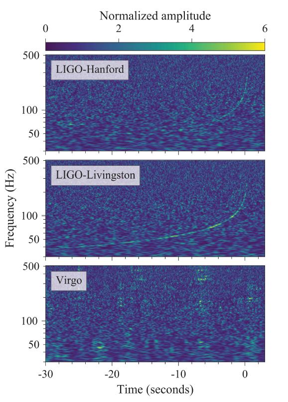
Figure 13. Time-Frequency Plots:The plots show frequency vs. time for the neutron star merger event GW170817. The two LIGO detectors show clearly the characteristic “chirp” upswing in the frequency as the objects merge. Image: LIGO Scientific Collaboration and Virgo Collaboration
The cosmic abundances of the elements beyond
the iron peak are much, much lower than the
elements below it, especially carbon, nitrogen and
oxygen. That is because the neutron capture
processes are far less efficient than core fusion.
As with the CNO cycle in hydrogen-fusing stars,
the nuclear physics (the propensity of atoms to
absorb neutrons, the decay timescales for
radioactive atoms, etc.) allows us to predict the
relative abundances of all the isotopes beyond
iron (and below, for that matter). In the vast
majority of cases, the predictions agree with our
observations, though there are a few discrepant
nuclei. Recent advancements seem to have
solved many of them.
To understand how this happened, there is one
more scenario by which elements beyond iron are
produced. This process was only recently
confirmed to take place, though it had been
suspected (even assumed) for some time. In an
effort that involved nearly the entire sway of fields
in observational astronomy, the merger of two
neutron stars was seen on August 17, 2017.
The event, designated GW170817, was tipped off when gravitational wave detectors (LIGO in the USA, VIRGO in Italy) saw the merger. Their data are depicted in Figure 13. The gravitational wave event coincided closely in time with a short gamma-ray burst (GRB170817A) detected by NASA’s Fermi Gamma-ray Space Telescope 1.7 seconds later in the same area of the sky. Because of the global alert system in place for GRB, many telescopes around the world and in orbit were quickly deployed to observe the new source, giving coverage over multiple bands of electromagnetic radiation. Even observations in neutrinos were attempted. An optical image of the fading afterglow of the GRB is sown in Figure 15, and Figure 16 shows an artist rendition of what the event might have looked like from a nearby vantage point.
These systems are formed when two massive stars in the same binary system die as
supernovae, leaving behind a pair of neutron stars. Generally, one of the stars dies before the
other one, and so the system for a while has a neutron star orbiting a normal star. Then the
second star dies, leaving a binary neutron star system. The neutron stars are small, as we have
mentioned earlier, and they contain the remnants of the core fusion processes of the original
stars, now all converted to neutrons. So how do they produce heavy elements?
As the stars orbit each other, they emit gravitational waves and slowly lose energy as a result.
During this phase the gravitational waves are weak and thus undetectable by current
instruments. Nonetheless, due to the energy loss the orbits shrink, and the stars spiral closer
and closer to each other.
This phenomenon has been observed previously in a binary pulsar system containing two
rapidly rotating neutron stars that flash radio pulses, something like a lighthouse, as they spin.
Their slow in-spiral was detected several decades ago, and the measured energy loss matched
precisely that predicted for loss from emission of gravitational waves. The system, called
PSR1913+16, provided the first indirect evidence for gravitational waves.
The decrease of the pulsar period with time is shown in Figure 17.
After many millions of years of in-spiraling, the neutron stars merge together; PSR1913+16 will undergo a similar merger at some time far in the future. When this happens, another titanic explosion occurs, a sort of mini-supernova, sometimes called a kilonova. The merger event creates a huge spike in the emission of gravitational waves, and almost immediately afterward, a flash of electromagnetic waves and a burst of highly beamed gamma rays. The former was seen by the gravitational wave detectors, and the latter was seen by Fermi and the other telescopes. No neutrinos were seen from this event.
Most of the matter of the two neutron stars comes together to form a black hole. However,
some of the material is thrown outward at high speed. This material can undergo nuclear
reactions via r-process neutron capture as outlined above. So, neutron star mergers produce
the same slew of r-process elements as happens in supernovae, but in greater amounts. In
fact, the neutron star merger process is now thought to dominate the cosmic production of the
r-process elements over supernovae. That means the gold in your wedding ring, assuming you
are wearing one, was probably produced in the merger of two neutron stars many billions of
years ago.
Summary
Looking up at the stars on a clear night from a dark location, they can seem cold, remote and
completely otherworldly. But they are not. Our increasing understanding of physics and
astronomy over the past two centuries has revealed that the lives of the stars are intimately tied
up with our own. We know they provide the chemical elements from which our own planet is
composed. We know that those same elements are incorporated into our bodies. And our
closest star, the Sun, provides the energy that powers almost all the life on our planet.
About five billion years ago, a massive star exploded. The expanding remnant from the
explosion, carrying with it the products of millions of years of nuclear fusion, crashed into a
nearby cloud and triggered its collapse. A new generation of stars, including the Sun, and
planets, was born. Without the contributions of that long-dead star, our solar
system, our planet, and we ourselves would not be here. The process of nuclear generation
continues to this day, with stars dying and seeding the cosmos with the raw materials for new
generations of stars and, at least in one instance of which we are aware, planets with life. In a
very real sense, we are starstuff. We are the children of the stars.
See the Additional Resources tab on the left.
Additional Resources
Line Spectra Resources
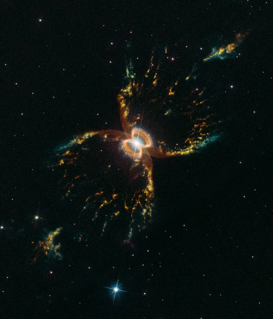
- Analyzing Light: Southern Crab Nebula – See how analyzing different parts of the light spectrum of the Southern Crab Nebula can help us infer the properties of the material inside.
- Analyzing Light: Starburst Galaxy M82 – By analyzing the different forms of light this galaxy emits, we can learn about its structure and what it is made out of.
Stellar Composition Resource
- Click here to see an example of a nearby star formation.
Summary Resource
- To see an example of a planetary nebula, the results of one such dying star, see ViewSpace’s multi-wavelength activity by clicking here.