
Introduction
Normal galaxies are, well, normal. They don’t have any of the extremely energetic things going on that Active Galaxies do. These are just your run of the mill galaxies.
Galaxies are large systems of stars and gas (and dark matter) that lie outside the Milky Way (the galaxy in which we reside). A typical large galaxy, like the Milky Way, is about 100 thousand light years across and contains 100 billion stars. Some galaxies are much smaller, less than 10% the size of the Milky Way, while others are more than ten times bigger. The nearest large galaxy to ours is the Andromeda galaxy (M31) which lies about 2.5 million light years away. It is part of our Local Group of galaxies, several dozen mostly small galaxies, along with Andromeda and the Milky Way, that comprises our local neighborhood. Most galaxies lie much farther away than Andromeda, and far beyond the bounds of the Local Group. The brighter ones in our night sky, which can be found in the Messier and New General catalogs, are typically tens of millions to hundreds of millions of light years distant. Much fainter galaxies lie beyond, stretching all the way back to the edge of the observable universe, with lookback times more than 12 billion years in the past. Use the links at left to explore some of the properties of galaxies and the observational characteristics we use to try to understand them.
Hubble’s Classification Scheme
The true nature of the galaxies was first convincingly demonstrated by Edwin Hubble when he showed that they are far outside the Milky Way. On the basis of photographic images Hubble suggested there are three major categories of galaxies. An example of each is shown below.
|
elliptical (E)
|
spiral (S)
|
irregular (I)
|
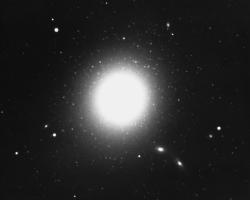 M87 |
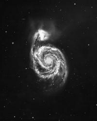 M51 |
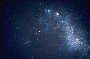 Small Magellanic Cloud |
| All Images NOAO/AURA/NSF | ||
Hubble expanded this preliminary classification system into what has now become known as the “tuning fork” diagram.
In this picture the ellipticals are distributed along the “handle” of the tuning fork, with decreasing ellipticity to the left. The spirals are distributed along two sequences. The splitting was necessary because of the presence of two apparently similar sequences of spirals. One contains the “normal” spirals, in which the spiral arms appear to come from a central galactic bulge. On the other, the “barred” spirals have spiral arms that appear to come from the ends of a linear bar-like structure that passes through the bulge.
The spirals can be placed in a sequence along which the arms become more open and the bulge becomes less prominent. This is indicated by the designations Sa through Sc (and SBa to SBc for barred spirals). Hubble thought this ordering might have been an evolutionary sequence, with objects evolving from tightly wound to a more open state. Thus, the Sa galaxies are still referred to as “early” galaxies while the Sc galaxies are referred to as “late” galaxies.
See the Additional Resources tab on the left.
Galaxy Evolution and the Tuning Fork Diagram
Hubble expected there should be an S0 class which formed an evolutionary bridge between the ellipticals and the spirals. Though he never detected such an object, the S0’s were added later by Hubble’s student, Allan Sandage. Sandage greatly expanded Hubble’s original system. Additional enhancements were also suggested by Gerard de Vaucouleurs, who added the class Sd as a class later than the Scs. An Sd galaxy has extremely open arms and a negligible or even non-existent nucleus.
We now know that the tuning fork diagram bears no relation to the evolution of galaxies, at least, not in the sense that galaxies evolve from “early” to “late” as envisioned by Hubble. However, we do see collisions in which two spirals can merge to form an elliptical, counter to the evolutionary development assumed by Hubble. This is only one way to form an elliptical though, and many galaxies likely form as ellipticals from the very start. Also, in the early universe we see that large ellipticals and spirals seem to be forming from small irregular galaxies; there is even strong evidence that this process continues to the modern day.
Spirals like the Milky Way and Andromeda have cannibalized small galaxies in the past, and they continue to do so (see the image of M51 at the top of this page). The Milky Way is currently in the process of devouring the Large Magellanic Cloud, one of its small companion galaxies. The well-known “globular cluster” Omega Centauri seems in fact to be the remnant nucleus of a small elliptical galaxy that has been consumed by the Milky Way. Furthermore, in several billion years observational evidence suggests that the Milky Way and Andromeda will collide and merge, eventually settling down to form a large elliptical galaxy. The image at right shows two galaxies engaged in a similar encounter.
Evidence now suggests that the process of galaxy evolution is one of titanic mergers and cannibalism, in striking contrast to the slow migration envisioned by Edwin Hubble early in the Twentieth Century. So even though his tuning fork diagram is not at all related to the evolution of galaxies, the classification scheme originated by Hubble is still a useful way to describe the current appearance of a galaxy, if not where it came from or where it might be headed.
Galaxies Observed in Multiple Wavelengths
We customarily classify galaxies and attempt to describe their morphological characteristics primarily on the basis of visual light images. This is in part a historical accident in that we first examined galaxies (spiral nebulae or elliptical nebulae) 200 years ago using visual inspection of telescopic images. Beginning 100 years ago photographic emulsions began to be used to record astronomical images. While the spectral sensitivity of photographic emulsions is slightly different from the spectral sensitivity of the eye, the two are close enough so that they are both commonly referred to as “visual light” images. Of course, it turns out that the visual-light region is the most advantageous one for studying galaxies in general since this is the region where stars (and hence galaxies) usually emit the most radiation.
However, as technological advances have made it possible to image astronomical sources outside the visible band, it has become apparent that some morphological structures are more pronounced in the IR, radio or even x-ray than they are in the visible. Indeed, some relatively featureless galaxies have revealed vast amounts of structure in non visible bands. For example, in spiral galaxies the dust scatters and obscures visible light while allowing IR, radio and x-ray photons to pass through relatively unimpeded. Furthermore, the dust becomes a stronger emitter of IR photons at the temperatures of the interstellar medium. As this technology has improved, we have come to recognize that a far clearer understanding of galaxies is possible when we observe both visible and non-visible photons.
See the Additional Resources tab on the left.
Galaxy Color
When we refer to galaxy color we are generally using it as a proxy for the stellar population. Early type galaxies like ellipticals do not contain cool gas or dust. As a result they do not form stars and are dominated by an older, redder stellar population. Spirals, on the other hand, do form stars and therefore have a younger, bluer stellar population mixed in with their underlying old disk population. This effect is not a large one, however, and most spirals are not appreciably bluer than elliptical galaxies.
Besides stellar content there are other properties that affect the color of a galaxy. One is the presence of dust. Dust will scatter short wavelength light while letting the longer red wavelengths through. Therefore, extremely dusty galaxies will appear red regardless of their underlying stellar population (this is the same process that causes the Sun to be redder at sunrise and sunset than at midday). Indeed, such dusty galaxies will often be undergoing extremely vigorous star formation, but their thick dust content blocks a direct view of their young, bright stars. Instead we may see that they have inordinate emission in the infrared, the result of the massive stars warming the dust and causing it to glow in the IR.
Sometimes a galaxy can be bluer than we expect given its morphology or stellar content. This will be the case for galaxies with extremely old stellar populations. Generally we think of old stars as being red, but if the stars are extremely old they would have formed before the galaxy had produced many metals (in astronomy, “metals” are all elements heavier than hydrogen and helium, and all those heavier than boron are formed inside stars). They will therefore be metal-deficient. The preponderance of atomic transitions for many of these elements is in the UV part of the spectrum. In stars with many metals the absorption in this region somewhat blocks emission there; much of the flux that would normally be emitted in the UV must come out at longer wavelengths, making these stars redder than they would otherwise be. On the other hand, low-metal stars are able to emit more light in the blue and UV parts of the spectrum, which somewhat diminishes their emission at longer wavelengths. While this is a small effect, it can subtly change the color of the stars in a galaxy, making it slightly bluer would be expected (actually, slightly less red is a better way to think about it).
So color is not always a simple thing. Generally a red galaxy will contain older, cooler stars. But in some cases there is more to it, either because of the presence of dust in the galaxy or because of low metal content.
Galaxy Spectra
Galaxies are studied mostly through the light they emit. When astronomers study an object, they often spread its light out into the constituent wavelengths or energies that the light contains. For visible light these are seen as different colors. The light is often displayed on a graph, with brightness plotted against wavelength. The brightness can also be plotted against energy or frequency… these are all basically equivalent. Such a plot is called a spectrum. Studying the spectra of astronomical objects is how many astronomers spend their time. This is because understanding an object’s spectrum is the key to knowing many things about it. Below we discuss some general features of galaxy spectra.
In addition to morphology, as described above, the spectra of galaxies can also be used as an aid in classifying them. The spectrum of a galaxy is produced mostly by the stars it contains, and so galaxies generally show the same spectral lines commonly seen in stars. Of course, the lines are broadened due to the galaxy’s rotation since, at any given moment, some stars are moving toward us, while others are moving away. These motions shift the position of the lines according to the Doppler shift formula. So one thing we can measure from the spectrum of a galaxy is the speed at which its stars move within it (which in turn allows us to measure its mass). But we can learn many other things about a galaxy from its spectrum. In particular, the presence of strong emission lines in a galaxy’s spectrum is a sign of star formation.
The spectra below at right are both taken from Parisi et al., 2009 (arXiv:09095345v1). Each is a plot of flux (in erg per square centimeter per second per angstrom) vs wavelength, here plotted in Ansgstrom units (1 angstrom is 0.1 nanometers, or 10-10 meters). To break this down, the plots show how much energy (in ergs) from the galaxy passes through each square centimeter of the detector during each second at each wavelength plotted (in angstroms). For reference, the bluest light visible to humans has a wavelength just short of 4000 angstroms, and the reddest light visible is around 7000 angstroms. So this spectrum runs from violet to just beyond the red part of the spectrum in the near infrared. Of course, the electromagnetic spectrum continues to shorter wavelengths (ultraviolet) and longer (infrared), but our eyes cannot see this radiation. Our detectors can, but those wavelengths have not been measured for these spectra.
You should keep in mind that these galaxies are at great distances, so their spectra have both been redshifted by the expansion of the universe. As a result, the lines shown are not at the wavelengths they would have in the lab. Despite these shifts, the patterns of the lines are the same as they would be in a nearby galaxy; the redshift effect only shifts the pattern. Redshift acts on each wavelength the same, shifting it by the same percentage as all other wavelengths.
See the Additional Resources tab on the left.
Galaxy Size
Sizes of galaxies are determined by measuring their angular extent on the sky and determining their distance.
Here s is the linear size, ø is the angular size in arc seconds, and d is the distance to the object. The units of s will be the same as the units of d. Of course, there are two difficulties with the practical application of this equation: (1) the precise determination of the angular size of a “fuzzy” object like a galaxy is difficult to make, and (2) the precise determination of the distance is also difficult.
The following results are typical measured values for galaxy diameters.
| dE dwarf ellipticals | 3 kpc |
| S spirals | 15 kpc – 20 kpc |
| E ellipticals | 60 kpc/td> |
| cD giant ellipticals | 2 mpc |
Here 1 kpc is a kiloparsec, and 1 mpc is a megaparsec. A parsec is approximately 3.2 light years.
Galaxy Luminosity, aka Absolute Magnitudes
Luminosities or absolute magnitudes can be determined for a galaxy by measuring its apparent magnitude and combining that with its distance. Here is it assumed that the flux of the galaxy diminishes as the inverse of the square of its distance from us (strictly, this is true only for point sources, but the methods used to measure galactic distances generally employ such sources). Just as for size, apparent magnitude determinations are difficult for galaxies since it is difficult to define the precise location of the “edge” for a nebulous object. In addition, corrections must be applied because of the attenuation by dust in our own galaxy, the attenuation due to dust in the external galaxy, the orientation of the galaxy in space (edge-on or face-on), and the K-correction due to the redshift of the galaxy.
The following results are believed to be typical absolute magnitudes.
| dE | -8 |
| S | -21 |
| E | -22 |
| cD | -25 |
Notice that the absolute magnitude for a dE galaxy is only one magnitude brighter than the absolute magnitude for the brightest single supergiant stars in our own galaxy and in the LMC. Just for reference, the absolute magnitude for the sun (a G2 main sequence star) is about +5, while the absolute magnitude for a star like Sirius (an A0 main sequence star) is about +1. A typical red giant star might have an absolute magnitude of about 0 (zero).
Elliptical Galaxies
Elliptical galaxies appear in the sky as luminous elliptical disks. Elliptical galaxies have more stars concentrated at their center than at their outer edges, but otherwise have little or no structure. The light distribution is smooth with the surface brightness decreasing smoothly outward from the center.
The actual light distribution of ellipticals is well represented as
Where C0 is the central brightness, and I(r) is the brightness at radius r from the center. These galaxies are classified by means of the elongation of the projected image. That is, if a and b are the major and minor axes of the projected ellipse, then the ellipticity class, Ec,
is a measure of the ellipticity. This quantity is observed to vary fairly smoothly from E0 to E7. Statistical studies indicate that the true shapes of the galaxies are uniformly distributed from E0 to E7. There is no indication of the presence of any dust in these galaxies.
cD Galaxies
This type of galaxy appears similar to the ellipticals, and they are sometimes referred to as giant ellipticals. The type was introduced by W. W. Morgan. The “c” refers to an old spectroscopic designation for supergiants, while the “D” simply stands for diffuse. The objects appear to have greatly extended envelopes and frequently exhibit structure and multiple nuclei near their centers. They may have sizes which are ten times larger than a normal elliptical.
cD galaxies are probably the result of two or more objects merging together, or of a larger object “swallowing” or cannibalizing smaller galaxies.
Irregular Galaxies
Irregular galaxies show no symmetrical or regular structure. Galaxies of type Irr I have resolved OB stars and HII regions. Irr II do not resolve into stars and are generally amorphous. Irregulars seem to contain a higher than usual concentration of dust and gas. Because of the dependence on resolution, it is impossible to distinguish between Irr I and Irr II for more distant objects.
Hubble described this class as lacking both dominating nuclei and rotational symmetry. In general, this class displays a lack of any organized structure. The suffix p, for peculiar, should generally be reserved for galaxies with obvious structure that has been distorted by the tidal interaction with close companions.
Lenticular Galaxies
Lenticular galaxies (Type S0) are intermediate between the E7 ellipticals and the Sa spirals. They are flatter than E7s and have a thin disk as well as a spheroidal nuclear bulge. When they are seen edge on they sometimes have the shape of a convex lens, so they are also called lenticulars. The disk components have a light distribution that falls off more slowly than in the ellipticals.
An S0 galaxy seen edge-on is very difficult to distinguish from an Sa seen edge-on. An S0 seen face-on is very difficult to distinguish from and E0. High quality images are necessary in order to discern the faint disk. Thus at increasing distances the identification of the S0s becomes increasingly more difficult.
S0 galaxies are disk galaxies, like spirals, but they have far less dust and gas than a normal spiral. It is possible that S0s are early type spirals that have lost their dust and gas as a result of tidal interactions with other galaxies. It is even possible that S0s are early type spirals which have suffered collisions. One clue to the nature of lenticular galaxies is that they are preferentially found near the centers of rich clusters of galaxies, where the intracluster gas would strip the interstellar dust and gas from a galaxy as it falls through the cluster.
Ring Galaxies
There are galaxies known to have very large ring-shaped structures beyond the nucleus. Some of these galaxies look almost like the planet Saturn, with their large prominent ring surrounding the nucleus. Sometimes the nucleus is nearly absent, so the only structure apparent is a large ring. In either case, these galaxies are termed “ring galaxies” and have been classified as R (for “Ring”). If an underlying spiral structure is discernible, the galaxy might be classified as S(R) or SB(R). Note that the upper case R is used for large ring structures beyond the nucleus, while the lower case r is used for ring structures features within or near the nucleus.
It has been suggested by some that ring galaxies are produced as a consequence of a galaxy-galaxy collision.
Dwarf Galaxies
Most of the galaxies with which we are familiar are bright and easily detected. However, the vast majority of galaxies in the universe are actually small and faint. They tend not to fit into the classification scheme as we have outlined thus far. The most common form for these galaxies appears to be elliptical, and since they generally contain little or no gas, they are as a class referred to as dwarf ellipticals, dE. In addition to being smaller than the bright elliptical galaxies, the dEs do not exhibit a bright nuclear region. Another classification used for dwarf galaxies is dIrr (for dwarf irregular).
De Vaucleures has proposed the term “compact” to designate the dwarf galaxies. Thus, one can encounter the designations cE, for compact ellipticals, and cI, for compact irregulars.Since these objects are faint, they can only be detected if they are relatively nearby. This in itself can present a problem because some dwarf galaxies are so sparsely populated with stars that they are difficult to distinguish from Milky Way foreground stars. Nonetheless, given the large numbers of dwarf galaxies that we find in the local group and in other nearby groups, these are likely the most common types of galaxies in the universe.
Spiral Galaxies
Spiral galaxies are either ordinary (S or SA) or barred (SB). Both types have spiral shaped arms, with two arms generally placed symmetrically about the center of an axis of rotation. In the ordinary spirals the arms emerge from the nucleus, while in the barred spirals the arms emerge near the ends of a bar-like structure which passes through the center of the nucleus. Both types are classified according to how tightly the arms are wound, how patchy they are, and the relative size of the nucleus.
Ordinary spirals of type Sa have smooth ill-defined arms that are tightly wound around a large prominent nucleus. The arms are wound so tightly they are nearly circular. The intermediate Sb galaxies have more open arms which are often partly resolved into HII regions and stellar associations. The nuclei of Sc galaxies are usually quite small and the arms are well extended and resolved into HII regions and clumps of stars. An Sd galaxy displays virtually no nucleus at all.
| Hubble described this sequence in the following manner: |
| “The arms appear to build up at the expense of the nuclear regions and unwind as they grow; in the end the arms are wide open and the nuclei inconspicuous. Early in the series the arms begin to break up into condensations, the [breakup] commencing in the outer regions and working inwards until in the final stages it reaches the nucleus itself. The “breakup” referred to is the appearance of HII regions and bright blue supergiants.” |
See the Additional Resources tab on the left.
Active Galactic Nuclei (AGN) Galaxies
Galaxies are huge collections of stars which are held together by gravity. Often, large galaxies have centers (also called nuclei) which contain supermassive black holes. Some galaxies appear active when large amounts of stars, gas and other material get fed into the black hole releasing matter and light away from the center. Depending on which orientation this process is viewed from, Active Galactic Nuclei can be observed as huge amounts of light of different energies which changes over time (but doesn’t usually repeat periodically like other variable objects). At first, these objects were given different names because astronomers didn’t know they were usually AGN viewed from different angles. Some of the most powerful objects in the Universe, studying AGN can help us understand how physics works at the extreme limits where huge amounts of matter and energy come together in small spaces. NASA’s Fermi mission has measured thousands of AGN and helped link these objects to the production of strange particles called neutrinos which are incredibly difficult to detect on Earth.
One of the general characteristics of Active Galactic Nuclei (AGNs) such as quasars, blazars, and Seyfert galaxies is that they seem to be variable in brightness. It is often assumed that most, if not all, AGNs are variable at some level. For example, virtually all of the AGNs observed in the Hubble Deep Field were determined to exhibit detectable variability over a period of two years. Furthermore, some categories of AGN known as BL Lacs, (refered to as blazars) are among the most extremely active variable sources known in the universe. Based on the limitations of the existing data and analysis, some systematic observational material would substantially improve our understanding of the nature of the variability of AGNs.
Variability studies of AGNs typically focus on one of three time scales. These time scales are related to the nature of the data and to the logistics and practical matters associated with obtaining astronomical observations. These time scales are not necessarily related in any meaningful way to physical process producing the variability. These time scales may be termed longterm, intraday, and microvariability.
| Time Scale | Typical time scale for viewing the data | Typical time resolution |
| Longterm | Several years or decades | Months or years |
| Intraday | Several days or weeks | Days |
| Microvariability | Several hours | Minutes |
Historically, longterm studies have been based on estimates obtained from photographic plate collections. In some cases data can be available for nearly a century, but the coverage is random and can have significant gaps due to economic and political circumstances. Data will normally be based on different photographic materials and processes plus different instrumentation (cameras and telescopes). At best the precision of the data can be a few tenths of a magnitude, but measurement uncertainties of a half magnitude or more are certainly possible. Any detected variability can be expected to be decidedly undersampled. Examples of AGN Variability Longterm data can be found for the objects linked in the table below.
| OJ 287 | AO 0235+164 | B2 1215+303 |
| B2 1308+326 | PG 0804+762 | PG 1001+054 |
| PG 1626+554 | PG 1704+608 | PKS 0754+100 |
Longterm observational programs are always difficult to maintain. The difficulties are based on the commitments required in interest, in time, and in funding. Several of the large scale survey programs that have been proposed by major observatories and institutions, in conjunction with programs such as the National Virtual Observatory could ultimately provide a uniform homogeneous database for significant longterm studies of AGNs. Until the time that such large scale programs are approved and initiated, a small scale network of dedicated observers can make truly significant contributions to the study of the longterm variability of AGNs.
Intraday studies of the variability of AGNs essentially compare the brightness of an AGN from one night to the next for a period of days. Such programs typically involve the intensive observation of a selection of a dozen or so objects for five or ten days. This can be the extent of a typical allocation of observing time on a medium-sized telescope. It is not uncommon for such telescope allocation to be repeated in six months or a year. This can provide a target sample distributed around the sky and can provide follow up observations for targets previously observed. Examples of AGN Variability Intraday data can be found for the objects linked in the table below.
Unfortunately, observing intraday variability for only a few days at a time will grossly undersample the true extent of such variability. For example, it is well known that AGNs undergo active phases and quiescent phases. Intraday variability would be expected to be different during these different phases and a few isolated observations may not be sufficient to indicate the true activity level. The effective average time resolution for such limited programs is more likely near 5 or 10 days.
Microvariability studies involve sitting on a single AGN for several hours and taking data as fast as possible with the available instrumentation. Using modern CCDs with medium and small telescopes, a large number of AGN are accessible with exposure times less than a few minutes. Thus, the brighter AGNs may be observed with a time resolution of about one minute. Of course, such a program requires the exclusive use of a telescope for a single object. Examples of AGN Variability Microvariability data can be found for the objects linked in the table below.
Since microvariability has been confirmed for vitrually all classes of AGNs, such observing programs can be exciting. Flares can occur over a period of hours or less, and rapid qusi-periodic oscillations have also been observed. Variability over periods of hours has been well documented for numerous AGNs. Microvariability studies can be attractive to professionals since for a limited commitment of time, if one is lucky, one is virtually guaranteed a publication. Do you feel lucky?All published descriptions of microvariability typically report that several objects were observed without positive results, and that even objects exhibiting variability on one night may have been monitored on several other nights with no indications of variability.
Quasars
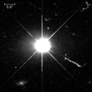
HST image of 3C 273. Note the starlike appearance and the jet of material being ejected toward the lower right.
In the late 1950s radio astronomers began compiling catalogs of radio sources. At that time, there were quite a number of radio sources which were not associated with previously known optical objects. The primary difficulty was that radio telescopes had poor resolution and large beam sizes so that it was often not possible to identify which of as many as several hundred faint stars was actually associated with a strong radio source. (Note that today this would not be a problem due to the advancements in resolution brought about by radio interferometric techniques). In 1960 one unassociated radio source (3C 48) was finally identified with a 16th magnitude stellar object. The identification was made when the moon occulted the radio source. Since this relatively strong radio source was associated with an object that appeared stellar, this category of objects became known as quasi-stellar radio sources (QSRS). This is the origin of the name quasar.
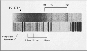
Discovery spectrum of 3C 273. Note the redshift of the hydrogen lines in the source relative to the comparison spectrum. The wavelengths of H-Delta, H-Gamma and H-Beta are, respectively, 410, 434 and 486 nm.
When a spectrum of this faint source was obtained it was observed to have strong broad emission lines which could not be identified with emission lines of known chemical elements. In 1963 the strong radio source 3C 273 was also identified with an inconspicuous 13th magnitude “star.” This object too exhibited strong emission lines which could not be identified. Eventually a sequence of emission lines similar to the Balmer series of hydrogen was recognized in the spectrum of 3C 273, but shifted far to the red. The red shift observed for 3C 273, z = 0.158, was greater than the highest known redshift for a galaxy. However, assuming this redshift, the remaining emission lines could readily be identified with the standard emission lines known. Because the emission lines identified in this way are the same lines known to be present in nearby galaxies, and because galaxies are the only objects known to have systematic large redshifts, quasars are generally believed to be extragalactic.
When Maarten Schmidt measured the spectrum of 3C 273 in 1964 it was the most distant object known… for about 15 minutes! Then his colleagues in the next office measured the spectrum of 3C 48, which gave z = 0.36.
If quasars are assumed to follow the Hubble law for distances, the large redshifts must correspond with large distances. Indeed, at the large distances implied by some quasar redshifts, a normal galaxy would be too faint to be observed. Thus, quasars would appear to be hundreds of times brighter than normal galaxies.
Quasars have now been observed with redshifts ranging from 0.06 to above 6.0. However, there are no nearby quasars, and the number of quasars increases with redshift. Since redshift is related to distance, objects with large redshifts are farther from us; it has taken their light longer to reach us, and so we see them from a time farther into the past. Since quasars are more numerous at high redshift, they must also have been more common when the universe was younger. Quasars have either disappeared during the present time or have changed their characteristics and evolved into less luminous objects. According to current thinking on the subject, all large galaxies went through an active “quasar” stage early in their existence, but have now settled down into quiet middle age. In support of this idea is the growing evidence that all large galaxies contain supermassive black holes at their cores… the same type of object thought to power quasars and other AGN.
Seyfert Galaxies
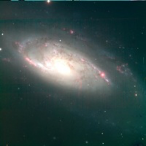
(Image: Seyfert (and LINER) Galaxy NGC 4258, Image: Soren Larsen, UC Lick Observatories)
Seyfert galaxies were first identified by Carl Seyfert in 1943. Initially they were classified as galaxies with broad emission lines. These galaxies also have unusually bright nuclei. Seyfert initially identified 6 such objects, and there are now approximately 90 known. They all appear to be spiral galaxies, and although 5-10% might be elliptical, the questionable objects all have extremely small angular sizes so it is difficult to discern any morphology. It appears that about 1% of all spiral galaxies might be Seyferts. It has been hypothesized that at least some spirals (or possibly all spirals) go through an active Seyfert phase under the proper conditions. Since most Seyfert galaxies appear to be in close binary galaxy systems, it may be that tidal interactions induce or even turn on the Seyfert phenomenon.
Since Seyferts generally exhibit both permitted and forbidden lines, the emission must be produced in different regions of the galaxy where different physical conditions prevail. Forbidden lines can only be produced in low density regions, whereas higher densities must occur where permitted lines are produced. In terms of their spectra there are now three sub-types of Seyfert recognized.
| Three subtypes of Seyfert galaxies |
|---|
| Type 1 |
| These are the “classic” Seyfert galaxies. They have extremely broad permitted lines of hydrogen. If the broadening is interpreted as being due to Doppler motions, the broadening corresponds to velocities of up to 5,000 or 10,000 km/sec! The forbidden lines (typically O II, O III, N II, S II, etc.) are only “moderately” broadened by 200-400 km/sec. For comparison, in an ordinary galaxy the escape velocity from the galactic disk is normally less than 300 km/sec. Of course, the emission lines in a Seyfert originate in the nucleus of the galaxy. |
| Type 2 |
| These Seyferts have “narrow” lines by comparison to the Type 1’s. The broadening rarely amounts to more than 200-400 km/sec (1000 km/sec in one case) and the permitted and forbidden lines have the same widths. |
| Type 1.5 |
| Some Type 1 objects are observed which have both broad and narrow components for the permitted hydrogen lines. A narrow emission peak seems to extend above the broad underlying emission line. |
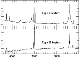
Example spectra of Type I and Type II Seyfert galaxies. Upper spectrum is actually more like a Type 1.5 (Note the narrow lines extending above the core of the broad lines). Image from Bill Keel’s Slideset on AGN.
The standard model for a Seyfert galaxy involves three components. First, a tiny central source of high energy ionizing photons, and then two distinct surrounding regions with different gas densities. Presumably, the inner region is the Broad Line Region (BLR) with high densities appropriate for the production of permitted lines. The velocities in this region must approach the 5,000-10,000 km/sec values deduced from the line widths. Because the broad lines are observed to undergo significant variability over periods of weeks or months, the size of this region cannot be much greater than a light month or so. This size corresponds to about 1011 km and is not much larger than the size of our planetary system. Gas densities in the BLR must be on the order of 1013-1015 ions/m3. Outside the BLR must be the Narrow Line Region (NLR) where the gas densities are low enough to allow forbidden line production. The scale size of the NLR must be about 102-103 times larger than the BLR. There are no observational reports of variability in the narrow lines.
Since there is no reason why permitted lines cannot be produced in the low density NLR, the existence of Type 1.5 Seyferts is totally understandable. Furthermore, slight differences in the widths of the narrow lines suggests that the density in the NLR decreases with radial distance from the nucleus. The critical densities for forbidden lines from different atomic species vary, and those lines coming from the least dense regions exhibit somewhat narrower lines.
The continuous spectra of Seyferts seems to be a combination of stellar, nonthermal, and IR emission from dust. Seyfert galaxies are not strong radio sources and the most sensitive radio surveys have detected only about half of the known Seyferts. Likewise, Seyfert galaxies are not strong X-ray sources.
Bright, star-like objects generally lacking any emission lines.
BL Lac objects are named after the prototype object which was first believed to be a variable star in our galaxy. However, because of its similarities to AGN, BL Lac is now believed to be an extra-galactic object. Because of their occasional wild variability, these objects are sometimes referred to as “blazars.” This name also alludes to the similarities these objects have with quasars.
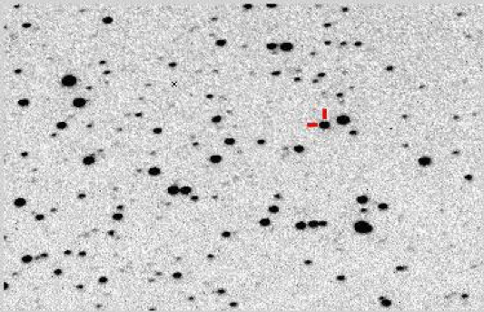
Image from: AAVSO – ask for permission (“Image of BL Lac, the prototypical “BL Lac” object. Credit AAVSO.”)
BL Lac objects have most of the following characteristics:
- Great and rapid variability in the radio, IR, and visible regions. Optical variability of up to 4 magnitudes is not uncommon. This amounts to a change in brightness of nearly a factor of 20, and a few BL Lac objects have been reported to undergo changes in brightness of a factor of 100. While variations of 10 to 30% have been noted from night-to-night for some objects, the larger variations usually take place over months or years.
- No emission or absorption lines… continuous spectrum only
- Compact radio source with non-thermal continuous spectrum extending into the IR and visible
- Stellar appearing optical source with virtually no structure. Some BL Lac objects reveal “fuzz” when observed with the largest telescopes. This “fuzz,” or faint nebulosity surrounds a point-like stellar appearing source.
- Strong and rapidly varying polarization
Approximately 40 BL Lac objects have been identified. Because of the virtual absence of emission or absorption lines, red-shifts are generally unknown. They are believed to be extra-galactic because of their radio properties and because of the “fuzz” observed surrounding some objects. The “fuzz,” when observed, seems to have a spectrum similar to that of an elliptical galaxy. A number of BL Lac objects are known in the vicinity of clusters of galaxies, so this provides indirect evidence in support of their extra-galactic nature.
Active Galactic Nuclei (AGN) Spectra
The spectra below at right are both taken from Parisi et al., 2009 (arXiv:09095345v1). Each is a plot of flux (in erg per square centimeter per second per angstrom) vs wavelength, here plotted in Angstrom units (1 angstrom is 0.1 nanometers, or 10-10 meters). To break this down, the plots show how much energy (in ergs) from the galaxy passes through each square centimeter of the detector during each second at each wavelength plotted (in angstroms). For reference, the bluest light visible to humans has a wavelength just short of 4000 angstroms, and the reddest light visible is around 7000 angstroms. So this spectrum runs from violet to just beyond the red part of the spectrum in the near infrared. Of course, the electromagnetic spectrum continues to shorter wavelengths (ultraviolet) and longer (infrared), but our eyes cannot see this radiation. Our detectors can, but those wavelengths have not been measured for these spectra.
This first spectrum is from a spiral galaxy. Notice the strong strong emission lines of oxygen (near 5000 angstrom) and hydrogen (just short of 7000 angstrom). Other emission lines are seen as well. Those from sulphur (S), nitrogen (N) and helium (He) are labeled. These lines are produced by hot, ionized gas clouds which are often seen in regions where stars are forming. As a result, the presence of these emission lines in a galaxy means it is forming stars. Only spirals and some irregular galaxies form stars, so just from looking at this spectrum you can tell that the galaxy is not an elliptical. The Roman numerals after the chemical symbols indicate the ionization state of that atom. OI refers to neutral oxygen, OII is singly ionized oxygen (loss of one electron) and OIII is doubly ionized oxygen (loss of two electrons). The presence of the helium emission lines indicate that this is no ordinary spiral galaxy. In fact, it harbors an AGN, and is therefore an active galaxy. This is also indicated by the broadening of the lines of hydrogen (especially H-alpha), nitrogen and sulphur. In addition to the emission lines, several different absorption lines are seen in this galaxy. The absorption lines will be discussed below in the description of the elliptical galaxy spectrum. You can click on these images to view a larger version if you wish.
This spectrum is from an elliptical galaxy. Notice the lack of most of the emission lines seen in the spiral galaxy, above. The only emission line seen is OII, which in this galaxy has been shifted to almost 5000 angstroms (it has a rest wavelength of 3727 angstroms). Like the example above, this is an active galaxy. If it were a normal elliptical there would be no emission lines at all. From the previous discussion of spirals you will deduce that the lack of emission lines in elliptical galaxies results from them having no star formation, and thus no ionized gas clouds. However, this last statement is somewhat misleading. Elliptical galaxies do contain ionized gas, but it is at temperatures higher than a million kelvin. At these temperatures the gas is so hot and highly ionized that it emits x-rays. We do not see any sign of this hot gas in the optical spectra shown. The gas in spirals, on the other hand, has a range of temperatures from only a few kelvin in the cores of molecular clouds, to about ten thousand kelvin in the ionized clouds responsible for the emission lines. You may notice that the absorption lines in this elliptical galaxy seem much more pronounced than the ones seen in the spiral spectrum. This is not really the case. The presence of the strong emission lines in the spiral spectrum makes the vertical scale somewhat compressed. The continuum (the continuum is the average value of the spectrum, ignoring emission and absorption lines) appears flatter in the spiral, and the lines seem to be not as deep as in the elliptical. In some spiral galaxies the emission lines are so strong that the continuum appears completely flat, but this is just an artifact of how we have chosen to plot the graph, with a linear vertical scale. If we blew up the vertical scale we would see that the continuum in both galaxies is about the same, with the same rough shape and similar absorption features. In both galaxies the continuum is produced by cool giant stars for the most part. So, aside from the emission lines from the star forming regions in the spirals, their spectra are similar to the spectra of ellipticals.
Additional Resources
Classification Resource
- Seeing Farther: Hubble Ultra Deep Field – An interactive site where you can see the evolution of galaxies through the Hubble Ultra Deep Field.
Multiwavelength Resource
- Neutral atomic hydrogen can be observed in the radio (1.414 MHz/21 cm) and yields views of galaxy interactions that are not at all obvious in other bands.
Spiral Galaxy Resource
- Click Here to go to ViewSpace’s light spectrum activity with two colliding spiral galaxies.