
On July 4, 1054, a “guest star” appeared in the sky, as noted by observers in China, Japan and possibly Europe and North America. The “guest star”, however, was not an actual star. It was a supernova. A supernova is a tremendous explosion that occurs when a massive star runs out of nuclear fuel and collapses. You can see the gas and dust left over from this explosion – the supernova remnant – if you point a telescope just a few degrees north and east of Aldebaran, the “eye” of Taurus, the bull. This supernova remnant is a faintly glowing cloud of cooling debris, known as the Crab Nebula. In the core of the supernova remnant, spins what remains of the original star – the Crab pulsar. Whirling around 33 times per second, this cosmic lighthouse sends out jets of particles and light that can be seen in videos made from images taken by NASA’s Chandra X-ray observatory.
Not all “guest stars” originate in massive stars, however. There is another type of supernova that was first envisioned by Indian scientist Subrahmanyan Chandrasekhar – after whom NASA’s Chandra X-ray Observatory was named. When smaller stars, like our Sun, run out of nuclear fuel, instead of exploding as a supernova, they eventually become a collapsed, cool object known as a white dwarf. If the white dwarf is orbiting another star, the white dwarf can gain mass by gravitationally attracting matter from its partner. And if it gains too much matter, growing heavier than the theoretical limit that was calculated by Chandrasekhar, it will collapse, ultimately creating a supernova explosion. These Type 1a supernovae all have similar properties, and hence predictable brightnesses. Each shines as bright as a `10^36`-watt lightbulb, and appears fainter at greater distances from Earth. Thus, by measuring the supernova’s brightness at Earth, we can determine how far away it is.
In the Build a Light Curve exercise, you will learn how to measure the brightness vs. time from an example Type 1a supernova. The peak brightness of a Type 1a supernova can be used to determine its distance. In the Hubble Constant exercise, you will measure the peak brightnesses of a collection of similar supernovae, and will compare the distances determined using this method to the recession velocities determined by measuring the redshift of a spectral line. The comparison will lead you to calculate the Hubble constant, which is inversely related to the age of the Universe!
The goal of this procedure is to obtain the relative brightness of a supernova which occurred in 2014 in the galaxy M82. Prior to the supernova, the star was unremarkable. As the white dwarf collapses, however, the stellar image will brighten significantly, and then fade. The peak brightness of this supernova will be used to determine its distance, in a subsequent activity. You can start to make these measurements yourself using the telescope images provided below. Each image contains the supernova, which will appear as a bright star. You will obtain the relative brightness of the supernova with respect to two companion stars.
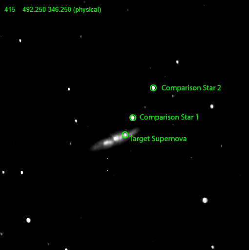
Below are two windows: the Finder Chart window below on the left shows an image of the target supernova and two comparison stars. In the window on the right, you will use a software tool called JS9 to perform the image analysis. First, you will select a region that includes the target star, and measure the brightness in that region. Then you will select each of the two comparison stars and measure their brightnesses. The comparison stars were chosen because they are known to have a constant brightness. By comparing the brightness measurement of the target to the average brightness of the two comparison stars, you will be able to tell if the target supernova has changed in brightness.
However, there is a limitation with this data analysis approach. – it cannot measure the true brightness of the target, only the relative brightness. Relative brightness is a number which can be close to 0.0 (zero, target is very faint), near 1.0 (one, target is near the average brightness of the comparison stars), or greater than 1.0 (target is brighter than the average brightness of the comparison stars). Measuring relative brightness for a series of images creates a plot called a light curve. Follow these steps to use a software tool called JS9 to create a light curve for the example supernova, which occurred in 2014 in the galaxy M82
1. Press the T1 (Time 1) Button to load the first Supernova image
2. Press the Zoom Button to zoom into the correct spot of the picture.
3. Press the LOG button to make it easier to see the stars. If you click and drag the mouse across the JS9 window you will be able to adjust the contrast of the image.
4. On the finder chart below, your target Supernova is in the small green circle closest to the bottom of the chart compared to the other circles.
5. Open the Magnifier Box by pressing the Magnifier Button.
6. Move the Magnifier Box so it doesn’t block buttons or boxes.
7. Press the Add Region Button to load in a circle that you will use to measure the brightness of the supernova as well as the brightness of the different comparison stars. Once you have clicked on the circle, use the arrow keys on the keyboard to move the circle more precisely. If you end up with more than one circle click your extra circle and press the delete key on your keyboard.
8. Drag the circle to your target supernova and click the Target Button.
9. Drag the circle to comparison star 1, as shown circled and labeled on the finder chart and click the Comp 1 Button.
10. Drag the circle to comparison star 2, as shown circled and labeled on the finder chart and click the Comp 2 Button.
11. Click the Plot Button to plot the relative brightness, which is the regional pixel count of the target supernova divided by the average of the regional pixel counts of the comparison stars. The plot is drawn under the finder chart and JS9 window.
12. Repeat these steps for each of the available Supernova images taken at different times, (T1-T5).
Finder Chart
Region Pixel Counts:
You are about to compare your relative brightness calculations for this Supernova in the M82 galaxy with those calculated by astrophysicists for many more images taken as the supernova brightened and then dimmed. Your relative brightness calculations will remain on the plot below in blue. The astrophysicists’ calculations will show in red.
Now that you have learned how to measure the brightness of a Type 1a supernova, you can proceed to use a collection of these “standard candles” to derive your own measurement of the Hubble Constant: the rate at which the Universe is expanding. In order to do this, you will analyze two types of data from each supernova: the lightcurve and the spectrum. For each plot of a supernova lightcurve, you will choose the brightest point and click on it. The value of the brightness you select will be entered into the answer box in magnitudes. Magnitudes are special units typically used by professional astronomers that get larger as objects become fainter. For example, a 14th magnitude star is about 2.5 times brighter than a 15th magnitude star.
Each supernova also has a second chart that shows its spectrum: how much energy is emitted as a function of the wavelength of light. After clicking the button labeled “Spectrum” click on the wavelength that corresponds to the lowest point in a Silicon absorption line near 6150 Angstroms. (One Angstrom is equal to `10^-10 m`.) The wavelength that you measure will be greater than 6150 Angstroms, because the expansion of the Universe will shift the absorption line towards longer wavelengths (“redshift”).
Now that you have selected the peak brightness (in magnitudes) and wavelength (in Angstroms), for each supernova, the numbers have been automatically filled in the table below. This table also does the rest of the calculations for you. First, the peak magnitudes are converted into distances by assuming the peak brightness of each supernova is the same. Then the wavelengths of the line minima are converted into recession velocities by measuring the redshift of the line. When the recession velocities (y-axis) are plotted against the distances (x-axis) , the slope of the best fit line in the plot is the measured Hubble constant. Hubble constants are typically measured in `km s^-1 Mpc^-1` . For each Megaparsec traveled, the expansion velocity of the Universe increases in km/sec. For example, a Hubble constant of `70 km s^-1 Mpc^-1` means that at a distance of `1 Mpc`, objects are moving away from us at 70 km/sec. At `2 Mpc`, the recession velocity would be 140 km/sec, and so on.
| Magnitude | Wavelength | D | Dist., Mpc | Dist., km | Redshift | Speed |
|---|
The equation that is written above is the best fit line from the table of measurements that you created.
The slope of the line is the Hubble constant.
The age of the Universe is related to the inverse of the Hubble Constant. Note that `1 Mpc = 10^6 pc`, `1 pc = 3.26156` light years, and 1 light year = `9.46` x `10^12` km. Therefore, with proper conversion of units, the Hubble constant can be converted into units of `s^-1` . The inverse Hubble constant therefore provides the approximate age of the Universe in seconds, which can then be converted into years (1 year = `3.154` x `10^7` seconds). Click the Calculate button and enter your value of the Hubble constant to calculate the age of the Universe from your measurements.