
Cookie Cutter Astrophysics: Beginning CCD Photometry
Some Technical Details about CCDs
A CCD is constructed in the same manner as a computer chip. The CCD detector is composed of an array of rows and columns of individual light sensitive elements or pixels. An incoming photon of light strikes the detector and produces electrons that are stored in the detector until they are read out. Built-in electronics will organize these electrons as charge packets and a computer can display and record these packets as a digital image. The resulting digital image is composed of numbers that correspond to the relative numbers of photons that struck the individual pixels. These numbers are generally called the “pixel values”.
The classic description of how this all happens was eloquently described in a paper by James Janesik and Tom Elliott of the Jet Propulsion Laboratory. This was first published as “History and Advancements of Large Area Array Scientific CCD Imagers,” by the Jet Propulsion Laboratory, California Institute of Technology, CCD Advanced Development Group.
Imagine an array of buckets covering a field. After a rainstorm, the buckets are sent by conveyor belts to a metering station where the amount of water in each bucket is measured. Then a computer would take each of these data and display a picture of how much rain fell on each part of the field. In a CCD the “raindrops” are photons, the “buckets” the pixels, the “conveyor belts” the CCD shift registers, and the “metering system” an on-chip amplifier.
Technically speaking, the CCD must perform four tasks in generating an image. These functions are:
- Charge generation
- Charge collection
- Charge transfer
- Charge detection
The first operation relies on a physical process known as the photoelectric effect – when photons strike certain materials free electrons are liberated. In the second step the photoelectrons are collected in the nearest discrete collecting site or pixel. The collection sites are defined by an array of electrodes, called gates, formed on the CCD. The third operation, charge transfer, is accomplished by manipulating the voltage on the gates in a systematic way so the signal electrons move down vertical registers from one pixel to the next in a conveyor-belt like fashion. At the end of each column is a horizontal register of pixels. This register collects a line at a time and then transports the charge packets in a serial manner to an on-chip amplifier. The final operating step, charge detection, is when the individual charge packets are converted to an output voltage. The voltage for each pixel can be amplified off-chip and digitally encoded and stored in a computer to be reconstructed and displayed on a computer monitor.
Even though stars are technically point sources of light, a real star image will have some physical size due to the blurring by the earth’s atmosphere (technically known as seeing) and the diffraction and interference of the light waves that produce the image. A real star image will appear as the so-called seeing disk. This pattern will be brighter at the center of the disk and approach the sky background at the edges of the pattern.
Cookie Cutter Photometry
Duration:
Introduce concepts: 1 hour
Perform activity: 1 hour
Essential Question: How can we measure the brightness of a star?
Science Concepts:
- Stars have different brightnesses, which can be measured using digital detectors
- Digital detectors measure brightnesses more accurately than the human eye
- Astronomers use the magnitude system to measure star brightnesses
Objectives:
Participants will…
- learn about digital images.
- learn about the astronomical magnitude system.
- understand how to determine brightness for astronomical objects.
- gain experience using logarithms.
Background Information
Digital Images
Digital images are produced by special detectors. The most common detector available today to produce digital images is based on the concept of the Charge Coupled Device (CCD). In addition to being the detector of choice throughout much of modern astronomy and astrophysics, CCD detectors are the detectors in consumer level digital cameras and video camcorders.
A CCD is constructed in the same manner as a computer chip. The CCD detector is composed of an array of rows and columns of individual light sensitive elements or pixels. Incoming photons of light strike the detector and produce electrons that are stored in the detector until they are read out. Built-in electronics will organize these electrons as charge packets and a computer can display and record these packets as a digital image. The resulting digital image is composed of numbers that correspond to the relative numbers of photons that struck the individual pixels. These numbers are generally called the “pixel values.”
When astronomers use CCDs to detect photons, they are usually focusing light from the astronomical object with a telescope. Even though stars are technically point sources (because they are so far away), atmospheric effects, as well as other optical effects, blur the star into a disk. Astronomers call this “seeing,” and the apparent size of the blurred star is called the “seeing disk.”
Notice that you can see the individual pixels in the star image, as well as in the background. The inner circle represents the region within which effectively all the light from the star has struck the detector. For determining stellar brightness this is termed the “analysis aperture.” If we add up all the pixel values in this analysis aperture we will have a number that represents the brightness of the star. (This number is ultimately directly related to the number of photons coming from the star that struck the detector during the time the exposure was being made.)
However, other sources of light also reach the pixels in the analysis aperture. We must correct our star brightness in the analysis aperture for this effect. For more information on this, see the section Background Correction below.
Here the height corresponds to the value at a particular pixel and the rows and columns correspond to the location on the detector. If we could actually construct a 3D model of this pattern (say, out of blocks or clay) and then weigh the part caused by the star we could also use this number (the weight) to represent the brightness of the star. Of course, we would also need to correct this approach for the contribution due to the background.
Background Correction
When making a measurement of a star’s brightness, we must be careful to correct for any other sources of light. These can contaminate the values of the star brightness. These sources include light from the sky and from the detector itself. Together these are called (for obvious reasons) “background counts.”
Even under the most ideal circumstances the sky is never truly black, that is, without any light. Of course, in an urban or even a suburban environment light pollution from artificial light sources will illuminate dust and molecules in the atmosphere. The atmosphere itself emits some light resulting from interactions of solar wind particles with the upper atmosphere. Another source is the integrated light from faint and distant stars. All of these sources from the sky are recorded by the detector, and are collectively called the “sky brightness.”
A final important source results from the detector itself. Even in the total absence of light a detector will produce electrons that get placed into the pixels. For an electronic detector this is termed “dark current.”
In order to accurately measure the brightness of a star, the observer must correct for these background counts. The “background annulus” formed by the inner and outer circles represents a region we can use to estimate the average background brightness reaching each pixel. This factor may be used to correct the pixel sum from the analysis aperture depending on the number of pixels in the analysis aperture.
In this exercise, you will determine a method of doing this, and then determine the brightness of a star using the magnitude system.
The Astronomical Magnitude System
Astronomers measure the brightness of stars, galaxies, and even the sky itself using the “magnitude system.” Historically, the magnitude system is based on a concept first introduced by the Greek astronomer Hipparchus in about 129 B.C. Hipparchus produced the first well-known star catalog in the western world. In this catalog Hipparchus ranked stars by what he called “magnitude.” Since brighter stars tend to look bigger, Hipparchus called the brightest stars he could see those of the first magnitude. Stars not so bright he called second magnitude. Using this system he called the faintest stars he could just barely see sixth magnitude. This basic system has survived to the present time.
Galileo forced us to change this system slightly. When Galileo used a telescope to view the sky he discovered there were fainter stars. As Galileo expressed his finding…
Indeed, with the glass, you will detect below stars of the sixth magnitude such a crowd of others that escape natural sight that it is hardly believable. … The largest of these… we may designate as of the seventh magnitude: Sidereus Nuncius, 1610.
A new term was introduced (“seventh magnitude”) and the magnitude scale became open ended. As telescopes became bigger and better astronomers kept adding more magnitudes to the bottom of the scale.
By the middle of the 19th century astronomers realized it was necessary to define a more rigorous magnitude system. It had been determined that a 1st magnitude star was approximately 100 times brighter than a 6th magnitude star. Accordingly in 1856 Norman Poigson proposed that a difference of five magnitudes be defined as exactly a factor of 100 to 1. Since at this time in the western world it was believed that all human senses were logarithmic, it seemed perfectly reasonable to define a magnitude difference between two sources in the following manner…
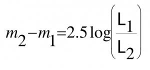
Here the Ls are the amount of light from object 1 (the bright object) and 2 (the faint object). This gives the magnitude difference between the faint object and the bright object. Keep in mind that fainter objects will have larger magnitude numbers and brighter objects will have smaller magnitude numbers. (Very bright objects will even have negative magnitudes). This relationship became known as Poigson’s rule. This rule describes how brightness measured by some instrument sensitive to light can be represented as astronomical magnitudes.
It is particularly convenient (and even easy) to determine the magnitude of a star with respect to a nearby star for which the magnitude is known. That is, we can determine the magnitude difference between an unknown star and a reference star or standard star with a known magnitude. This type of magnitude determination is termed “differential photometry.” Of course, in the final analysis all magnitude determinations are differential since the stars themselves (or at least a set of standard stars) effectively determine the entire magnitude system.
Materials for each participant:
- Clay model star field (modeling clay or Play-Doh)
- Plastic knife
- Pencil
- Triple beam balance or kitchen scale (for measuring mass)
- Ruler
- Paper plates
- Wax paper
Procedure:
- Pre-class: Prepare the clay star field models for each group of participants. Have them read about CCD detectors for homework.
- In class: Go over the vocabulary. (digital image, pixels, CCD, background, photometry, astronomical magnitudes). Stress that the clay models are representations of the light striking the detector. The thicker (or higher) the clay, the more light reached that particular part of the image. Also stress that virtually all astronomical measurements are relative (or differential) with respect to some known standard objects or sources. Discuss with the participants the concept of a pixellated detector. Also discuss the magnitude system, giving them examples of magnitudes of different objects in the sky. Have participants calculate a few magnitude differences given star brightness measurements (say, in number of electrons produced, of the volts produced
by some detector). Instructors may need to help participants make a connection between the height of the clay model star fields and brightness. A good example would be topography maps for mountains. - Post-class: Look at some digital images of astronomical sources. Zoom in to see the pixels. Demonstrate the use of software used to analyze astronomical images.
Preparing the Clay Star Fields
Option 1: Instructor prepares the star field models.
For best results the mass of the clay or dough should be about: Be sure to record accurate masses of each star.
- larger star ~40g
- smaller star ~15g
- background should weigh out to be ~155g
Start with three fingers of modeling clay. Flatten it out using a pencil, a rolling pin, or your fingers. Make the sheet about 6 inches by 6 inches and about 1/4 inch thick. The sheet does not need to be perfectly flat or smooth. Then take a strawberry sized piece of clay. Form this clay into a cone. Measure and record the mass of the cone so you know what to expect for results. Lightly press the cone onto the sheet with the flat side of the cone down. Take more clay, of a different size, and form another cone. The second cone should be either larger or smaller than the first cone. Measure and record the mass of the second cone. Lightly press this second cone onto the clay sheet. You now have a model star field with two stars. Of course, you could add another star or two if you wish.
Option 2: Instructor prepares the cones that represent the stars. Students prepare the clay sheet that represents the background brightness. Instructor then adds the stars.
Option 3: Each pair of students or student team prepares a model star field. Students then trade models with another team. Each student team must record the measurements of their star field that they create for their classmates.
Activity Results:
The goal is to determine the magnitude difference between two model stars. Students must measure the mass of each model star. This includes determining how much mass is being contributed by the background and subtracting this background for the final results. The ratio of the masses for the model stars can then be used in the magnitude difference equation to compute a magnitude difference. If the masses of the star cones are measured before being placed on the clay sheets the true value for the magnitude difference that students should obtain can be known in advance.
Note: The students are not allowed to simply pull or separate the stars from the flat surface. You must encourage the students to figure out how to “subtract the background” from the star.
Extension Activities:
- Use binoculars or small telescopes to measure the brightness of some variable stars. The AAVSO provides excellent resources for such activities:
http://aavso.org - Obtain digital images using a local telescope system with CCD detector. Local amateur astronomers often have telescopes and CCDs that could be used to obtain some images. It may be possible to arrange a demonstration of the equipment and to obtain some images. Local universities or colleges may also have astronomy programs and may be willing to provide demonstrations and images.
- Obtain digital images using a remote robotic telescope system. Several organizations maintain robotic telescope systems and allocate at least some time for educational purposes. Such organizations include the Global Telescope Network (GTN), Telescopes In Education (TIE), and Hands On Universe (HOU). Several companies and organizations maintain telescope systems which may be reserved and used for a modest fee.
- Analyze astronomical images to determine magnitudes for variable sources. University researchers and research organizations may have image data that students could learn to reduce and analyze. Some organizations, such as the GTN, maintain image archives of variable objects that could be analyzed as student projects.
Lesson Adaptations:
Visually impaired students could touch the star model and describe what they feel.