Observing Strategies

Plan Your Observations
Poisson Statistics – Root n Noise
Obtaining Good Calibrations
Obtaining Good Science Images
Naming Your Files

1. Observe When Objects are High in the Sky

This might seem obvious, but you should always plan your observations before arriving at the telescope. You certainly don’t want to
show up for your observing session only to find that your intended object sets an hour after the sun does. Or worse, find that it set
an hour before! If this is the case it just means that you are observing that object too late in the year… of course, some transient
objects, like comets and supernovae, don’t give us a choice in this regard. But fixed objects are always nicely placed in the sky for
viewing at some time during the year (assuming we are not trying to view a southern sky object from the northern hemisphere!). You can
use the object’s
celestial coordinates to figure out when to observe
it. The thing to remember is that an object will be transiting (at its highest altitude) when the local sidereal time (LST) matches the
object’s right ascension (RA). This notion is best understood in terms of a simple relation:

HA = LST – RA

Figure 1. This plot from the XEphem package shows the altitude (degrees) of several AGN as a function of time (in hours) through the night. Similar plots can be made with other software packages. These plots are valid for GORT, which has a latitude around 38 N. They were made for the night of February 20.

Click on image for larger version.

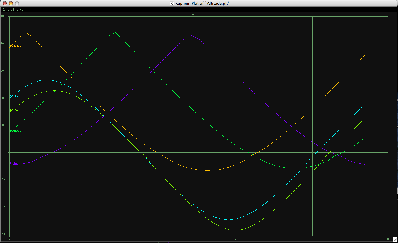
This states that the hour angle of an object of given right ascension increases with time, and in fact is the difference between its
RA and the LST. If terms like hour angle, local sidereal time, right ascension
and altitude are mysterious, look them up in an introductory astronomy text, or use the link for celestial
coordinates above to learn about them. It is useful to understand how celestial coordinates work before you plan your observations. To
get a general understanding of the night sky and the motions of objects in it, have a look at the fine set
of Astronomy Notes by Nick Strobel.

Of course, knowing when your objects will transit is only part of the information you need. It is also necessary to know when they
will rise and set. For example, if two objects both transit at the same time, but one is low in the sky when it transits and the other
is high , which should you observe first? If you look at the rising and setting times for each object you will find that the first one
(the one that transits low) will rise after the second and set before it. If you plot the altitude for each object vs. time you will
see that the low-transit object is mostly quite low in the sky the entire time. This makes it imperative to get the low-transit object
during or close to its transit time if possible. The other object will be high in the sky for several hours before and after transit,
so you are much more flexible in when you can observe it. The amount of flexibility will depend on the latitude of your site and the
declination of the objects in question. Have a look at the image above for an
example of what a plot of altitude vs. time looks like for several objects.

Finally, you should consider more than just transit, rise and set times because you cannot actually observe an object for the entire
time it is above the horizon. Most objects are best observed when they are no more than 45 degrees from the zenith. At lower points
atmospheric distortions will often seriously degrade the data. The amount of degradation will vary from location to location, and it
also varies with time. The general rule is that objects that transit high in the sky should not be observed when more than 3 hours of
RA from transit, either east or west. For objects that transit low in the sky these limits might have to be tightened
considerably. Again, these are rough guidelines. Some observing sites will be much better than this, others will be worse. And of
course, short term atmospheric conditions like haze or clouds will also have an effect.

2. Moon Phase and Observing

The Moon is one of the darkest objects in the sky. It reflects only about 11% of the sunlight it receives back into
space. Nonetheless, you have probably noticed that a moonlit night is much easier to navigate than a moonless one (discounting the
effects of artificial lights from cities and street lamps, of course). The Moon, especially when near full, causes the sky background
to increase enormously. As a result, if you will be observing faint extended objects like galaxies or nebulae, you will want to plan
your observations for a time when the Moon is below the horizon. All GTN objects are fairly bright point sources. These sorts of
objects suffer far less from the effects of moonlight, and so the Moon will often not be a worry for them (but see the discussion of
noise below, as sky brightness is one source of noise). But if you want to get a great shot of that lovely spiral galaxy, plan to do
it when the Moon is down.

3. Software Aids to Planning Your Observations

Many astronomical software packages can give you invaluable information for planning your observations. For instance, they can plot
the altitude vs. time of a sky position through the night. They can also give you
the phase and position of the Moon. An excellent package to perform these tasks
is Xephemeris, by the Clear Sky
Institute. Xephemeris is freely available from the web. For a modest charge you can buy it on CD, along with a manual on how to
run the software. Additional object catalogs and installation support are included with the purchase of the CD. Xephemeris runs on
Unix-type operating systems, which means various Unix and Linux distributions, FreeBSD and MacOSX. It does not run natively on
Windows, but you can run it using Windows plus one of several virtual machines. See the Clear Sky Institute website for details. Other
options for Windows users include
The Sky from Software Bisque,
and Starry Night. Versions of these packages will also run natively on the Mac. A
similar program is the open source package Stellarium, which is really designed to be run in a
planetarium. However, it does have some of the functionality of the other packages, and it runs on numerous platforms. See product websites
for details.

Poisson Statistics – Root n Noise

All measurements contain “noise.” Sources of noise include random fluctuations in the electronics of the detector, in
the sky, and in the source being observed. While these fluctuations are random, they do often follow a fairly simple rule: The
mean deviation from the average number of counts in a pixel (called the standard deviation) is equal to the
square root of the total number of counts in that pixel. Therefore, we expect that the total noise will increase with time as
the number of counts gets bigger. Statistics that follow this sort of relation are called Poisson Statistics, and they are
fairly simple to deal with. We will not go into a detailed description of how to deal with Poisson Statistics here (You’re
welcome!). Below we describe only enough for you to be able to use some general statistical ideas to guide your thinking when
planning a set of observations. See books like Data Reduction and Error Analysis for the Physical Sciences by
P. R. Bevington and D. K. Robinson, or Statistical Treatment of Experimental Data by H. D. Young for details of Poisson
Statistics if you want to learn more.

The Root of the Matter

Noise increases with time. This sounds like a bad thing because it means we get more noise the longer we observe. Of course, we all
know that longer exposures actually give better images, not worse ones. This is because we also get more signal over time,
not just more noise, and the signal increases faster than the noise does. The signal usually increases linearly with time, so
if n is the signal (number of counts in a pixel) we can write n =Rt, where R is the rate at which counts
accumulate (counts per second, say, assumed constant), and t is the time. In the simplest case, the noise is just the square
root of the number of counts. We can take the ratio of the signal to the noise (S/N) to find that

So the signal to noise ratio actually increases with time, albeit sloooowwwwly, with the square root of the time. Since we
generally want as high a signal to noise as possible, it might seem that we want to observe for as long as possible. But there is a
trade-off. We don’t actually get a lot of additional S/N for a large investment of time. For example, we get only about 40%
more S/N if we double the time, and only about 3 times more if we increase our exposure time by a factor of 10! Thus, we must weigh
our desire for high S/N against the practical limitations of observing time. In general we observe only as long as we need to in order
to obtain high enough S/N to satisfy our science goals.

That was a very brief, and very simplified, overview of Poisson Statistics. Now let’s see how you should employ these ideas when
planning your observing session.

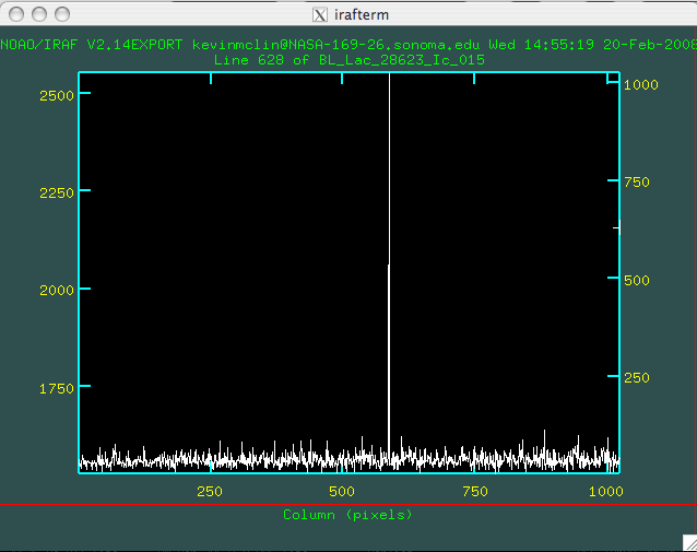
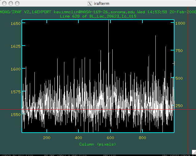
1. Take Lots of Calibration Data

Extracting meaningful science from your images requires that you have
good calibration images. Without them your data are nearly worthless from a
scientific standpoint. There are some standard tricks that you can use to ensure you obtain high quality calibrations. The first trick
is to note that calibration images are not bound by the rules regarding observing time. Calibrations can often be taken for hours at a
time during the daytime. What’s more, some of the calibrations can use a bright light source, enabling a large number of counts per
pixel (and thus a large S/N) in a short amount of time. This is important because we want to have as high a S/N in our calibrations as
we can get. We will have to combine the noise from our calibration images with that of our science images during our analysis phase, and
we want to make the calibration noise contribution as small as possible. Ideally we would like it to be so small as to be utterly
negligible. We do this by taking lots and lots of calibration data. However, we don’t just take very long exposures during our flats
and darks. There is a better way. Read on.

2. Stack Individual Calibration Images

There is an unavoidable problem encountered when using a CCD to take long exposures. Inevitably, you will find that some of
your pixels will be hit by cosmic rays (high energy charged particles from space). These will be obvious on the images: you will
see a saturated pixel, or sometimes two or three, surrounded by completely normal pixels ( see Fig. 2, above). This happens because a single cosmic ray packs more than enough energy to fill the well in a
pixel. However, its path usually only passes through one pixel. These pixels add unwanted noise to your data. How to deal with
them? Stack several images on top of one another!

Image stacking does not actually involve physically stacking your images. It means that you combine many images into one. There are
several ways you can do this. Common ways are summing (simply adding the corresponding pixels in many images to obtain a final image
which is the sum of the combined images) and averaging (basically, this is the same as summing, but with the added step of dividing
each pixel value by the number of images combined). Both of these methods have their uses, but if you are trying to get rid of cosmic
rays, then the best way to combine your images is to do a median combine. In a median combine you use the median value from each pixel
value, rather than the average or the sum. This has the advantage over the other two methods of being insensitive to large outliers –
like cosmic rays (it’s the same reason that Realtors use the median home price rather than the average home price to characterize a
neighborhood… they don’t want the statistic to be swayed by a lone $20 million mansion on the corner!). Most astronomical software
packages will have predefined functions that allow you to combine images in any of these three ways.

One additional word about median combine: it works better with an odd number of images. This is because the way to find the median of
a set of values is to order them (lowest to highest, say) and then choose the middle value. Obviously, if you have an even number of
values, then there is no middle value. In that case many software packages average the two innermost values. This is perfectly fine,
but it’s an extra step and takes some time. If you have lots of images to work on, then having an even number will take slightly longer
to work through because of this extra step. Do yourself (and your computer) a favor and just get into the habit of always taking an
odd number of images.

What about the statistics when you median combine? You’ve combined many images, presumably all having slightly different numbers of
counts. When you median combine them, you will get an image with about the same numbers of counts in each pixel as the combined
images. Does this mean that your S/N is roughly the same as before you combined them? No! If that were the case there would have been
little point in combining them. The S/N has increased by a factor equal to the square root of the number of images combined into the
final image. So if you combined 9 images your S/N in each pixel will be 3 times higher (because the noise is three times smaller) than
you would get from the pixel counts alone. If you combined 16 images (but you wouldn’t have because 16 is not an odd number) you would
get 4 times the S/N. Simple, no? Again, we will ask you to trust us on this. If you want to see where it all comes from you should
read references on statistical treatment of data such as the two we have recommended above.

Just as for your calibration images, you should take an odd number of images so as to facilitate the removal of cosmic rays
later. Three should be the minimum number of images taken for each target, though 5 is usually better (recall that the noise decreases
like the square root of the number of images taken). With very fast readout times on modern CCD cameras you will not pay a high
penalty in reading out multiple images as was the case a few years ago. Don’t forget to apply these same rules to any standard stars
you will be observing. In fact, you should treat them with as much care as you would your science images, since without good standard
comparisons your data will lose much of their value.

	3C273_V_60_1x1_001.fits 
	3C273_V_60_1x1_002.fits 
	3C273_V_60_1x1_003.fits 
	3C273_V_60_1x1_004.fits 
	3C273_V_60_1x1_005.fits 

These file names tell us not just the name of the object observed, but also important things like the filter used, the exposure and
the pixel binning. Without meaningful names like this you would have to look in the header of each image if you wanted to get this
information. Very tedious indeed, especially with many dozens or hundreds of images, and in a single night of observing the number of
image files you generate can easily grow into the hundreds. You should use meaningful names for your science images and do the same
for your calibration images. See the page on obtaining calibration images for
suggestions on how to name your calibration files. It is also helpful to put all the files for one night’s observing into a directory
that uses the date for its name. That way you automatically know on which night any given science image or calibration image was made.

1. Plan your observations to enable all your targets to be observed when as high in the sky as possible.
2. Plan with the phase of the Moon in mind, if appropriate.
3. Get plenty of calibration data either immediately before or immediately following your observation run (or both!).
4. Remove cosmic rays by median combining an odd number of images. This goes for both calibration images and science images.
5. Keep your science goals in mind. They might require (or allow) the modification of any of the above.
6. Use meaningful names for the files containing your science and calibration images, and put them in a directory named for the night
   of the observations.

If you follow these steps your data will be as good as they can be, and your science results will be correspondingly good.