
Overview
Image calibration refers to the process of removing artifacts from your data that are due strictly to the imaging system used, in this case assumed to be a telescope and CCD camera. Calibration must usually be completed before you can perform any science analysis with the images. There are three parts to image calibration:
- Obtain the calibration images
- Process the calibration images
- Apply the calibration corrections to the science images
- Obtaining Flat Field Images – These are used to correct pixel sensitivity variations across the chip.
- Obtaining Bias Field Images – These are used to subtract the chip bias signal, a constant signal in all images.
- Obtaining Dark Count Images – These are used to correct for dark count accumulation, which is caused by thermal motions within the detector.
Capturing Images Of The Night Sky
You will generally need three different kinds of calibration images. These are called flat fields, bias images and dark images, or often just flats, biases and darks for short.
For each night of observing you should acquire a set of calibration images to correct for artifacts that result during the CCD imaging. CCD control software has settings for each of the image types discussed above. Be sure to set the control software with the correct type of image flag so that the information can be properly written to the image header. If you will be binning your images, then you should be sure that your calibration images are binned the same way. For instance, if you will be taking your science images using 2×2 binning, take your calibration images 2×2 as well. The same goes for other binning configurations (including 1×1!). The control software for your camera will allow you to set image types, binning and a meaningful base name for the images, like flat, bias or dark. Check your camera or software documentation to see how to set these values.
There are additional calibrations that are sometimes needed, but they are generally not required with modern CCD cameras and will not be covered. If you have a cryogenically cooled CCD then you can probably skip the dark correction step. However, such systems require liquid nitrogen for cooling and are typically used only on professional grade telescopes.
See the Additional Resources tab on the left.
Flat Fields
Your flats are used to correct pixel-to-pixel sensitivity variations across the CCD. As such, they should reflect only variations in the chip itself and not any brightness variations across the sky. There are two methods that are most often used to create a set of flat fields. The first, called twilight flats (or sky flats), are images of the sky taken under twilight conditions. The second method, called dome flats, employs a reflective smooth screen illuminated by artificial lights. This screen, generally mounted on the inside of the dome, provides an evenly illuminated surface to image with the CCD. Either of these methods can be used to obtain a satisfactory set of flat fields, and which of them you use is up to you. Dome flats are certainly more convenient, but some people think that they are not as accurate as a good set of sky flats. There are even some observers who insist that “night sky flats” are the best way to go. These are flats that are made as the night sky tracks across the field of the telescope while the tracking motors are turned off. Regardless of which method you decide to use, you must take a set of flat fields for each filter you will use in your observations (be sure to label them with the name of the filter – something like vflat_001.fits, bflat_001.fits, etc. – so that you will be able to keep track of them). Also, be sure to set the image type to flat in your CCD control software, and to set the proper binning.
Twilight Flats
Twilight flats must be obtained just after sunset or just before sunrise when the sun is a few degrees below the horizon. Some people like to obtain flats at both times and then combine them all into one master flat field in each of their filters. The general strategy is as follows: For each of the filters you will be using in your observations, take an image of the sky under twilight conditions such that you almost (but don’t quite) saturate the chip. For instance, if your CCD pixels saturate at 65,535 counts, then you want to set your exposure time such that you are getting around 60K to 62K in each pixel. You don’t want to approach the saturation value too closely because then you will saturate the most sensitive pixels in the array. However, you still want to get as many counts in each pixel as you can (see the discussion of Poisson Statistics on the Observing Strategies page).
There are two complications with obtaining twilight flats. The first is that you will have to adjust your exposure time for each filter, since the sky has a different brightness in the different bandpasses and the CCD has different sensitivity in each as well. This would not be such an issue if it weren’t for the second complication, namely, the Sun is setting (or rising if you are making the flats in the morning). This means the sky level is constantly changing in all filters. One way to circumvent this is for the telescope to track the sun down (or up) as you make your flats. Another way is to adjust the exposure time, either up or down, in each filter as the sky brightness changes. Both of these complications can be overcome, however, what you have no control over is that there is only a short time, perhaps 20 minutes, in which you can obtain twilight flats. Rather than deal with the complications of twilight flats many people opt to make dome flats instead.
Dome Flats
Dome flats are made by taking an out of focus image of a white screen that is mounted inside the dome. The screen is illuminated by a diffuse light source that has good spectral coverage (for the filters you will use). Two advantages should be immediately apparent. First, the illumination of the light source is constant, so the same exposure can be used for each exposure. Second, the lamps can be left on for a long time, enabling the acquisition of many, many flat fields in each filter. With dome flats it is possible to write a script that will automatically direct the telescope to take as many flats in each filter as one would like (within reason). It is possible to automate the acquisition of twilight flats too, but it is much harder. Because they are so convenient, most observatories put a lot of effort into creating a system to make good dome flats.
If you want to check to see how well your dome flats are working, simply “flat correct” them using a set of twilight flats taken on the same night. If the dome flats are good, the result of this correction will be a completely flat image.
See the Additional Resources tab on the left.
Bias Images
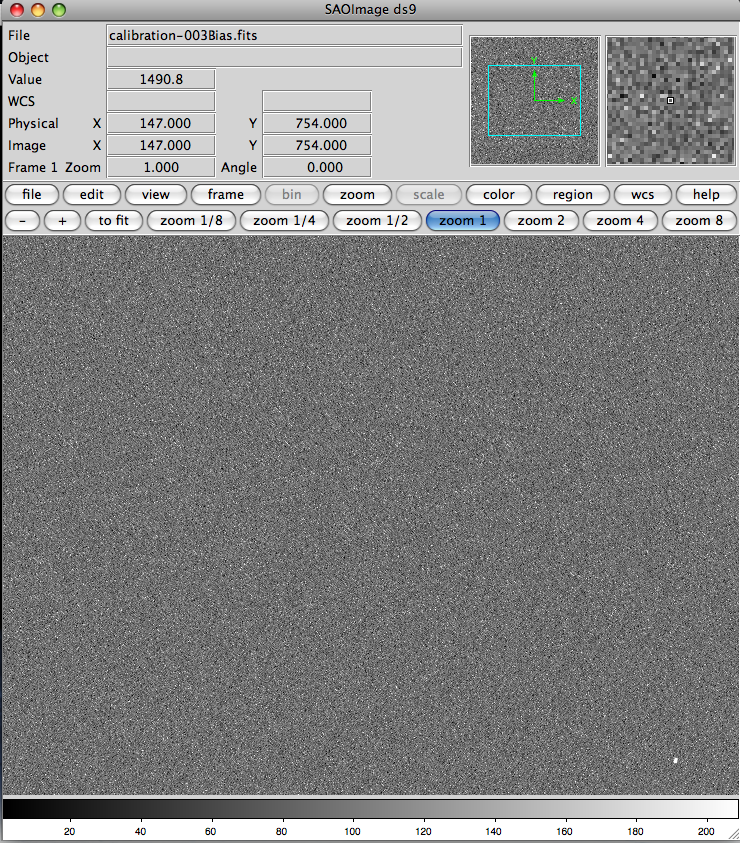
A bias image (sometimes also called a “zero”). Biases are quite smooth, as indicated by the image. Click on image for a larger version
Bias images are used to subtract the bias level for the CCD. The bias level is a nearly constant count level for the chip, often around 1600 counts. Biases are much easier to make than flats. They are obtained simply by recording an image without opening the shutter and with a zero second data acquisition time. Basically, they are zero-second dark images (see below). You should take many, many biases. They should be given names like bias_001.fits, bias_002.fits, bias_003.fits, etc. Take an odd number of bias images. Usually you can make bias images by setting the image type in your CCD control software to bias and then telling the controller how many images to take. Be sure the binning is set to the proper value to match your science images.
See the Additional Resources tab on the left.
Dark Images
Dark images are just what they sound like… images taken while keeping the CCD in the dark. This is accomplished by accumulating data while the camera shutter is kept closed. In most CCD cameras, counts will accumulate even when no light hits the detector. These counts come from random thermal motions of the atoms in the crystal of the detector. By cooling the chip with liquid nitrogen these motions can be diminished to the point that the thermal motions are so small that the dark counts become negligible. However, such cameras require hardware that most amateur telescopes lack, and for this reason we assume most GTN members will make dark images.
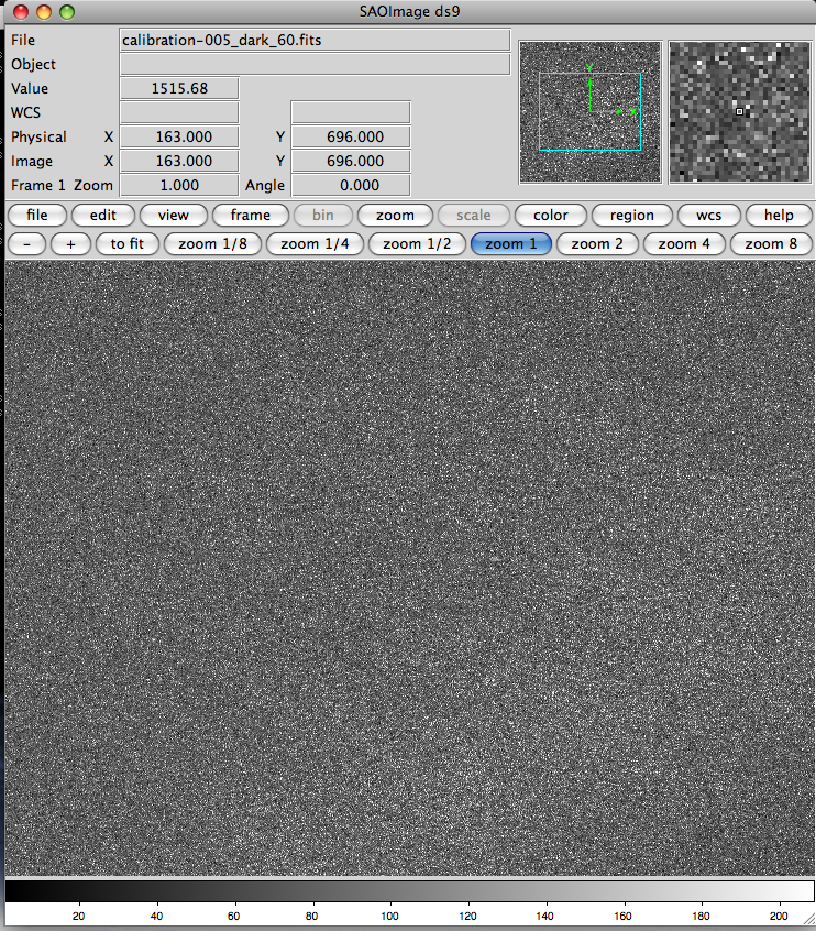
A dark field image, 60 second exposure. The level in a dark image will typically only be slightly higher than a bias. Click on image for a larger version.
In your CCD control software set the image type to dark. You will also have to set the exposure times for your darks. If you will be making 60 second science exposures, then you want to make darks with at least 60 seconds worth of dark count accumulation. If you will make 120 second exposures, then your darks should be at least that long. If you want to use 120 second darks with 60 second science exposures you can scale the dark counts down, though we caution that there is debate about whether this is a good thing to do. However, you cannot scale 60 second darks up for 120 second exposures. Many people simply make sure that they have dark exposures that match the exposure time of any science images they will be making. Feel free to use either strategy. If you really want to see if there is a difference, try reducing your images both ways and check the results.
Just as for biases and flats, you want to get as many dark images as you can (at various exposure times if you wish). You can then combine the darks of a given length into a single master dark for that exposure time. Darks can be made in the afternoon before your observing run, or in the morning following it, so it is not difficult to get lots and lots of them. Like bias images, darks can be made in great abundance, so you should get as many as you can. Take an odd number, just as you would for other images, so that you can median combine them into your master darks. Be sure to set the binning so it will match your other images.
Calibrating Your Images
Image calibration consists of removing effects due to variations in pixel sensitivity, bias and dark counts from your images. This process has three steps, outlined below.
- Bias Subtraction – The chip bias is an innate background in your chip which shows up in all images. You want to remove this because it artificially elevates the counts in every pixel, whether exposed to light or not. This is what your zero-second dark exposure images are for… your bias images. The bias will vary from chip to chip, and even from night to night. Typically the bias level is around 1500 ADU. Subtract the master bias from each of the other calibration and science images in turn. After the bias is removed, most CCD detectors will require the dark counts to be subtracted. That is the next step.
- Dark Subtraction – Unless your camera is cryogenically cooled (typically such cameras sit in a dewar filled with liquid nitrogen) you will have to apply a dark subtraction. From your dark images you can see that even in zero light conditions, counts accumulate over time. This rate of count accumulation varies with time and temperature, and will vary from detector to detector. Usually the accumulation of dark counts is linear with time, though for very long exposures this ceases to be true. Usually you can scale a dark exposure downward (never upward) to match the exposure length of the science image you are correcting: Just multiply the master dark by the ratio of the science image exposure time to the exposure time of the dark. You will have to do this for each exposure time in your science images, making a scaled dark for each. If you are doing these operations manually, or with software you have written yourself, you should copy the dark to a temporary file, and then use that file for the scaling and subtraction. That way you will not lose your master dark file. Astronomical software packages all do this for you, so you will not have to worry about this step if you use one of those. Of course, you can also take a set of dark exposures for each set of science images, matching the exposures of each while at the telescope. In any case, once you have a dark image that matches the exposure of each science image, subtract the darks from the corresponding science images, thus removing the dark count contribution from your science images. Now all that is left are the flat corrections.
- Flat Correction – Each pixel in a CCD acts like a nearly independent light detector. As such, the chip can exhibit slight variations in sensitivity from one pixel to the next. This causes brightness variations across the image. In addition, defects or obstructions in the optical path can cause illumination fluctuations on the chip. This is the source of the infamous “dust donuts” seen on uncalibrated CCD images. Flat fielding corrects the image to a “flat” sensitivity… one that does not vary from pixel to pixel. To do this, take your bias and dark subtracted flat fields and compute the mode of the pixel values for each of them (some people prefer to use the median). Divide each flat field by its mode, creating a new normalized flat. Now divide your processed science images by this normalized flat. This procedure will lower artificially high pixels and raise artificially low ones, “correcting” them all to a uniform sensitivity level.
Until you have completed all the steps above you might want to work with copies of your raw science images. That way, if something goes wrong along the way you will have your original files to fall back on. Once you have successfully completed all the calibration steps you can discard your raw images to save space (they are presumably still available somewhere, but you will not need them for subsequent reductions). When you have completed all the calibration steps above, you must (typically) combine your science images… you should take multiple exposures of each target in whatever filters you will use so that cosmic rays can be easily removed, just as was done for your calibration images. If you do not have multiple images of each target you can skip the steps about stacking your science images.
- dark_30_001.fits
- dark_30_002.fits
- dark_30_003.fits
- …
- dark_60_001.fits
- dark_60_002.fits
- dark_60_003.fits
- …
- dark_120_001.fits
- dark_120_002.fits
- dark_120_003.fits
- …
Processing Your Calibration Images
We assume that you have a set of calibration images and science images sitting on your computer in some directory. You might have acquired these images yourself at the telescope, or they might have been made for you. In any case, you will have to get a set of calibration images made at roughly the same time as your science images in order to reduce your data. Using calibration images made much much before or much after your science data is not recommended. To begin with, put all of your calibration images (flats, biases and darks) into a separate subdirectory called calibration. This is not absolutely necessary, but it helps you keep track of what files are where. You must first combine your calibration images into a set of master images (master bias, master darks, master flats). You do this for two reasons. The first is that combining images reduces the noise in your data (The noise is inversely proportional to the square root of the total number of counts, and combining images results in more counts). The second reason, is that combining helps remove cosmic ray hits that might be contaminating some of your images. The master set of calibration images will be applied to your science images. We describe how to produce these images in the chapter tabs above.
Flat Fields
You should have a set of flat fields for each filter used for your science data. As with your other calibration images, the flat fields should ideally have been taken during the same observing session as the science images, though in a pinch you can probably get away with using calibration files from an adjacent night. Dust spots, chip sensitivity and dark counts can change over time, so using the wrong calibration images can actually increase your errors rather than decreasing them. Depending on your project this may or may not matter.The first thing to do with your flats is to collect them by filter and merge the flats from each filter into a single flat field image file for that filter. For instance, if you have 11 flats in each of BVRI, you should merge your eleven B flats into a single flat field for the B images. Merge the eleven V flats similarly into a single flat for the V images, and so on. Call your merged flat images something meaningful, perhaps Bflat.fits, Vflat.fits, Rflat.fits and Iflat.fits for images in BVR and I, respectively. Exactly how you accomplish this merging depends on what software package you are using. Consult the documentation for your package to learn how to use it to merge your images.

| A Note About Combining Images |
| Many people median combine their images. That means that the images are compared, pixel by pixel, and the median of the pixel values from the images is used for the resulting combined image. Other ways to combine images use the average of the pixel values or simply the sum. You may use whichever method you like, it’s just a matter of preference. However, median combining has the advantage that it is insensitive to large outliers from the mean (whereas both the sum and the mean are quite sensitive to large outliers). Therefore, median combining is better able to remove cosmic ray hits. Since cosmic rays can be a large source of noise for long exposures (and occasionally even for short ones), getting rid of them is a good idea. Cosmic ray hits are easy to spot in your images because they create an area of only one or two pixels where the chip is saturated: astronomical objects will never do this. Fortunately, such features are easy to remove by median combining several images.Median combining is simpler if you use an odd number of images, so we recommend that you always take an odd number of each type of image (for both your calibration and science images). |
When you have created your master flat fields, move them into a directory with your science images. You are ready to move on to your other calibration images.
Bias Images
You should have acquired a set of bias images during your observing run. Note that some people (and software packages) call bias images “zero” images because they are taken for zero seconds and without opening the camera shutter. You must combine these biases (or zeroes) too. Again, using a median combine is recommended to remove outliers. When you have combined your biases into a single image, perhaps naming the result something like “bias.fits” you should move it into the directory where your science images reside. Note that there are counts in these bias images. Even though the exposure time was zero seconds and the shutter was never open, you still see a non-zero count level. These counts are intrinsic to the chip. They are in all the images you take, including flats, darks and science images. You will use your master bias image to subtract these counts from your other images.
Dark Images
The last type of calibration image you will need is called a dark image. These are made by taking an “exposure” with the shutter left closed. In this case, counts will accumulate due to thermal motions of electrons in the detector even though no light hits the detector. These “dark counts” also accumulate when the shutter is open, so they add a background noise signal to your images. You will use your dark images to remove these thermal counts.Some people like to have one dark image for each exposure time in their science data, where the dark exposure matches the science exposure. Other people take a set of long darks, combine them into a single master dark, and then scale that to the exposure time needed for each science image during the dark correction step. Again, the “best practice” is a matter of preference. One thing that is not in question is that whatever dark image you use for a given science image, it should be of at least as long an exposure as the science image. You can scale the counts of a long exposure dark image down to match the exposure of a science image, but you should never scale the counts in a dark exposure up. (By scaling we mean that you multiply the dark image counts by the ratio of the exposure time in your science image to the exposure time in the dark image; this ratio should never be greater than one.).Separate your darks by exposure time… hopefully they have names that make this easy, something like
|
|
|
|
These would be for darks of length 30, 60 and 120 seconds, respectively. You should combine each of these so that you end up with a single file for each exposure length. Again, median combining is the recommended way to merge them. You then end up with dark30.fits, dark60.fits and dark120.fits. When you have created a dark for each exposure time, move them into the directory with your science images and your other master calibration images. You are ready to calibrate your CCD science images.
Additional Resources
Image Capture Resource
- To learn how these images are used with your science images see the pages on data reductions.
Dome Flats Resource
- To understand why it might be desirable to obtain dome flights, see the Observing Strategies page).
Resource for Capturing Bias Fields
- See the Observing Strategies page for an explanation of why you should take an odd number of bias images.